
INTRODUCTION
Abstract
This is a natural language text analysis of the contents of user Posts contained in the Steem blockchain. The analysis is performed with the R language and supporting libraries.
Posts are an important part of the Steem ecosystem and arguably the backbone of the social platforms (portals) that use it.
While traditional BI analysis is useful, it tends to be time series analysis of discreet data (e.g. trending population size and transaction volume). This analysis differs by trying to mine insights about psychographic, sentiment or cultural influences.
Rich and thriving social platforms should exhibit thematic word patterns associated with cultural groups or topics of interest. This is a first attempt at identifying these patterns.
The content of a Post includes URLs, emojis, dingbats, images as well as text in numerous different character sets and encodings. These contributions come from a wide variety of different technologies from smart phones to PCs from Windows to Android, each with text encoding nuances. Emoji for example are poorly supported by MS Windows, and will originate from iOS, Android and OSX users. While emoji is limited by platform they appear in sufficient volume to generalize over the population (sampling theory).
Bias & Exclusions
The Steem blockchain contains high volume of marginal-value content such as food pictures, meme gifs, bible quotes, inspiration and motivation pictures. While users may enjoy consuming this content, it offers little value in NLP or text analysis. Extracting meaningful content from these binary images and videos is an image process exercise and out of scope of this analysis. Therefore I've excluded several high ranking categories/tags of predominately multi-media content.
I've also excluded Korean and Spanish which rank highly and I apologize to those native speakers for my ignorance of their language.
Target Selection & First Data Draw
The first dataset is drawn from Q1 of 2017. At the time of this analysis this is the most recent available from Steemdata.com which had been undergoing engineering work.
With this code we select all the Categories and count the number of posts they contain.
mdb <- mongo(collection="Posts",db="SteemData",url="mongodb://steemit:steemit@mongo1.steemdata.com:27017/SteemData")
cats<- paste('[{ "$match": {"created": {"$gte": {"$date": "2017-01-01T00:00:00.00Z"}, "$lte": {"$date": "2017-03-30T00:00:00.00Z"} } } },{ "$group": { "_id": { "category" : "$category" }, "Post Count" : {"$sum" : 1 } } }, { "$project": {"_id": 0, "category": "$_id.category" , "Post Count" : 1 } } , { "$sort":  { "Post Count": -1 } }]', sep="")
categories<- mdb$aggregate(cats)
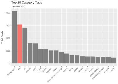
The dataset returns 9,463 distinct category tags. The average number of posts per category is 13 (the median being one). Somewhat surprisingly the 3rd Quartile is two posts, indicating the vast majority of tags are an empty wasteland with all the action going on in this top 20 or so. Given the rather generic nature of these top tags and the low averages, we can assume niche and specialized communities are few and far between (with top quartile exceptions like #steemsilvergold and #blockchainbi.
As mentioned above we exclude multimedia and non-english categories. The #Life category appears to offer sufficient Post volume for text analysis.
Target Acquisition & Second Data Draw
The second dataset extracts all the Posts tagged to the #Life category.
mdb <- mongo(collection="Posts",db="SteemData",url="mongodb://steemit:steemit@mongo1.steemdata.com:27017/SteemData")
# Extract Jan 2017
raw1<- mdb$find(query='{"created": {"$gte": {"$date": "2017-01-01T00:00:00.00Z"}, "$lte": {"$date": "2017-01-31T00:00:00.00Z"} },"category": {"$eq" : "life"} }', fields='{"_id":0, "body":1}')
# Extract Feb 2017
raw2<- mdb$find(query='{"created": {"$gte": {"$date": "2017-02-01T00:00:00.00Z"}, "$lte": {"$date": "2017-02-28T00:00:00.00Z"} },"category": {"$eq" : "life"} }', fields='{"_id":0, "body":1}')
# Extract Mar 2017
raw3<- mdb$find(query='{"created": {"$gte": {"$date": "2017-03-01T00:00:00.00Z"}, "$lte": {"$date": "2017-03-31T00:00:00.00Z"} },"category": {"$eq" : "life"} }', fields='{"_id":0, "body":1}')
I have to break the data into three sets (one per month) due to my crappy, underpowered 10 year old macbook.
The query takes 23.63 seconds to run and returns,
- Month 1: 2432 Posts
- Month 2: 2316 Posts
- Month 3: 2905 Posts
Browsing the content of the raw data for Month 1 shows it's pretty messy. Much of the kanji and foreign language is going to have to be filtered out (coerced to UTF-8 encoding) for analysis, reducing our dataset further.
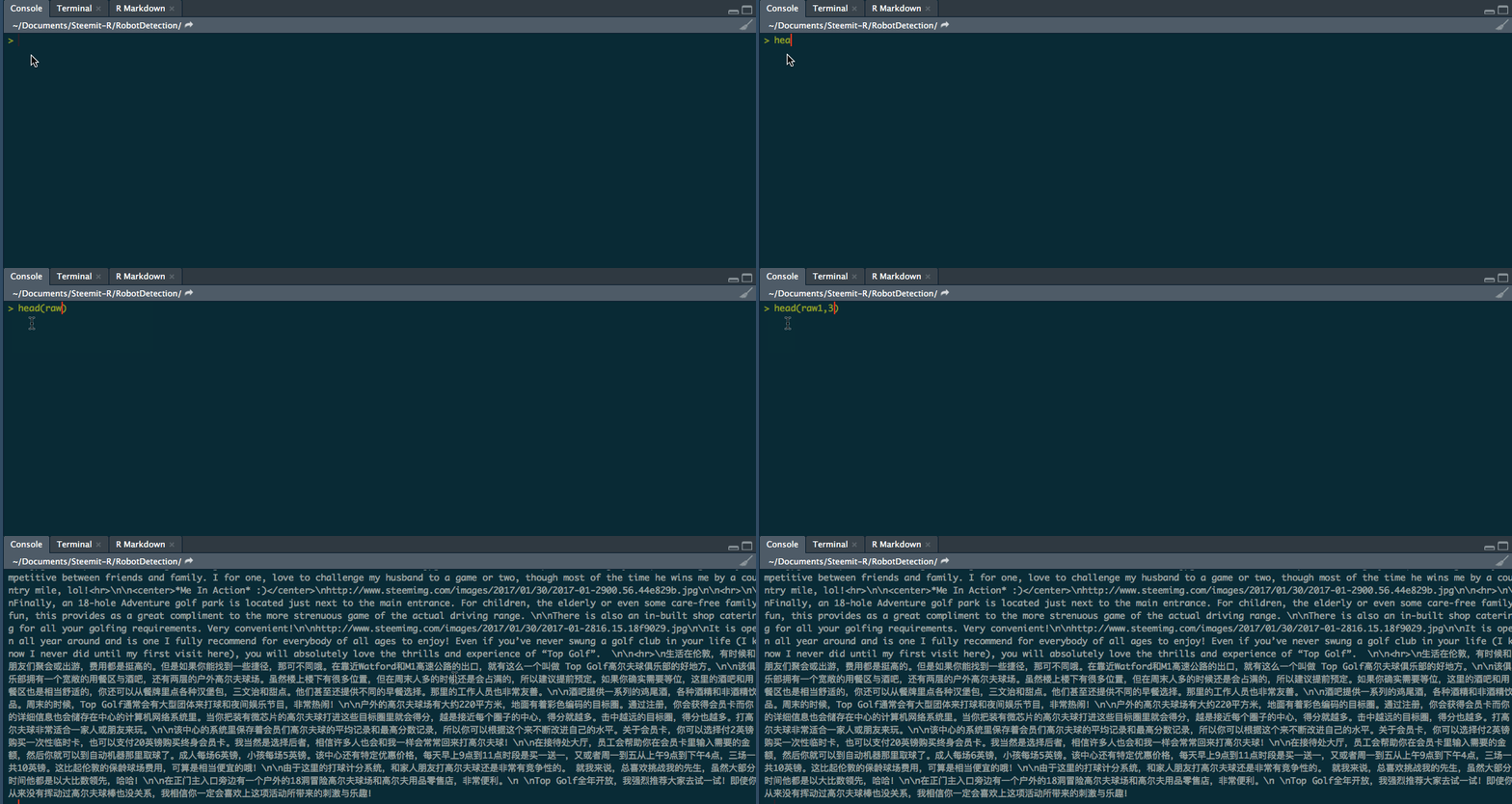
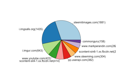
There is a large volume of non-printing meta elements including hyperlinks. These links are leaking traffic out of the Steem ecosystem to other inernet destinations.
This code will extract the URLs, pull out the fully qualified domain names (FQDNs) and count them.
  urls1 <- rm_url(raw1, replacement = " ", extract=TRUE, trim=FALSE, clean=TRUE)
  urls1 <- domain(urls1[[1]])
  urls1 <- as.data.frame(urls1, stringsAsFactors = FALSE)
  names(urls1) <- c("domain")
  urls1 <- sqldf("SELECT [domain], COUNT([domain]) AS [link count] FROM urls1 GROUP BY [domain] ORDER BY [link count] DESC LIMIT 50")
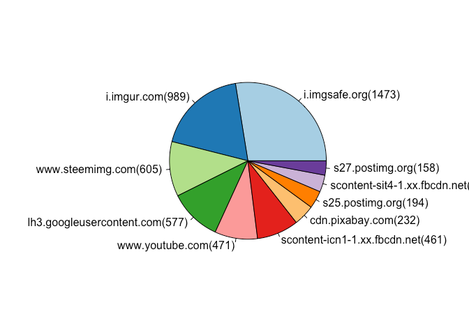
January Top Traffic Referral Destinations
The Top 10 are mostly image and video hosting sites, with a Content Delivery Network (CDN) in the mix. Nothing too surprising here with no significant changes month on month.
February Top Traffic Referral Destinations
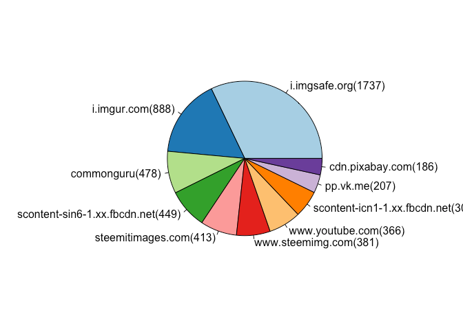
March Top Traffic Referral Destinations
Building a Document Corpus
Before further analysis, we want to preprocess our collection of texts and purge these URLs. We can use the Quanteda package to do this. While not perfect it will make a pretty good effort.
raw1.1 <- rm_url(raw1, replacement = " ", extract=FALSE, trim=FALSE, clean=TRUE)
raw2.1 <- rm_url(raw2, replacement = " ", extract=FALSE, trim=FALSE, clean=TRUE)
raw3.1 <- rm_url(raw3, replacement = " ", extract=FALSE, trim=FALSE, clean=TRUE)
We can now bring the the processed text into a document Corpus; a data structure designed for text analysis. We repeat the code below three times on each dataset resulting in a separate Corpus for Jan, Feb and Mar.
# Load cleansed posts into a data.frame
  cps1 <- as.data.frame(raw1.1)
# Assign a sequence id to each post
  cps1$id <- seq.int(nrow(cps1))
# Assign friendly column names
  colnames(cps1) <- c("text", "id")
# Swap/Reverse the column positions
  cps1 <- cps1[c("id", "text")]
# Build a document Corpus
  Corpus1 <- quanteda::corpus(cps1)
The Jan Corpus contains 1,478,770 words (of which 58,433 are unique) and 48,434 sentences.
The Feb Corpus contains 1,419,230 words (of which 56,802 are unique) and 40,146 sentences.
The Mar Corpus contains 1,353,873 words (of which 55196 are unique) and 44,815 sentences.
We observe more words were written in Feb despite having two fewer days than Mar. Incidentally, other analysis suggests user account growth between these two months too. More users contributing fewer words is a curious anomaly.
Creating a Document Frequency Matrix (DFM)
With our three Corpi we can now perform some basic text processing. Specifically we eliminate "Stop Words" and punctuation. Stop words are those with little meaning, such as "and", "the", "a", "an".
Some Steem specific Stop Words are also removed. These included stray html tags, css elements, line breaks as well as Steem vocabulary. Given the relative youngness of Steem it was clear users want to talk about the platform. Without removing them, these words consistently appear as the most frequent terms, drowning out any #Life related posts.
This preprocessing takes about 25 seconds.
# Define some Stop Words
  steem_stops <- c("steem", "steemit", "resteem", "upvote", "SBD", "n", "s", "t", "re", "nbsp", "p", "li", "br", "strong", "quot", "img", "height", "width", "src", "center", "em", "html", "de", "href", "h1", "h2", "h3", "960", "720", "en", tm::stopwords("en"))
# Create a DFM and further preprocess
  dfm1<-dfm(Corpus1, tolower=TRUE, stem=FALSE, remove=steem_stops, remove_punct=TRUE)
# Cal and sort Word Frequency
  dfm1.1 <- sort(colSums(dfm1), decreasing=TRUE)
  dfm1.1.wf <- data.frame(word=names(dfm1.1), freq=dfm1.1)
January Top 10 Word Frequency
    can   will    one people   like   time   life   just    get    day
   3807   3660   2985   2887   2802   2794   2708   2524   2019   1850
February Top 10 Word Frequency
    can   will   time people    one   like   life   just    get    day
   3555   3056   2581   2563   2560   2452   2126   2107   1839   1576
March Top 10 Word Frequency
    can   will    one people   time   like   life   just    get     us
   3700   3201   2934   2762   2660   2622   2340   2339   1834   1708
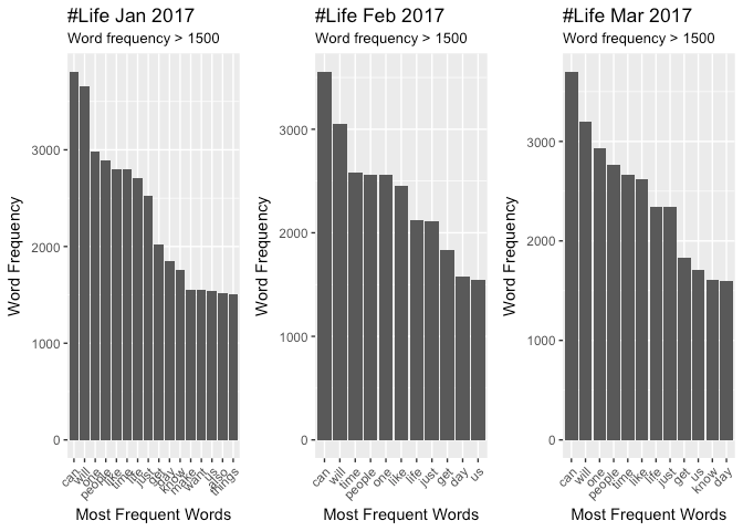
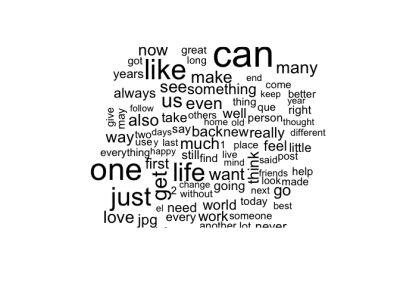
It appears similar words reappear consistently with "can" being the consitently top verb. Collective nouns ("people", "us") are common but without action verbs we can't infer what these persons might be up to. I was expecting to see words like "yoga", "meditation", "happiness", "gratitude" etc.
Phrasal verbs might give more insight but this will require assembly of bi-grams. Additional Time and more serious Compute resources would be required for this.
Assess Topics with Latent Dirichlet Allocation Model (LDA)
In an attempt to get more insight to what users are thinking and feeling, we can attempt to mine out word groupings with a word cluster analysis. We hope these word clusters can identify Topics and Themes.
library(topicmodels)
dfm1LDAFit<- LDA(convert(dfm1, to = "topicmodels"), k = 5)
get_terms(dfm1LDAFit, 10)
After playing around with different parameters (number of groups and words per group) we find no obvious themes in the clusters.
January Topic Clusters
    ##       Topic 1  Topic 2 Topic 3 Topic 4     Topic 5
    ##  [1,] "one"    "life"  "can"   "can"       "will"
    ##  [2,] "will"   "make"  "will"  "people"    "can"
    ##  [3,] "life"   "us"    "just"  "time"      "time"
    ##  [4,] "time"   "one"   "us"    "like"      "want"
    ##  [5,] "day"    "now"   "day"   "know"      "people"
    ##  [6,] "people" "much"  "like"  "get"       "just"
    ##  [7,] "just"   "like"  "think" "one"       "make"
    ##  [8,] "get"    "know"  "get"   "see"       "like"
    ##  [9,] "always" "can"   "go"    "even"      "now"
    ## [10,] "really" "way"   "one"   "something" "good"
February Topic Clusters
    ##       Topic 1  Topic 2  Topic 3     Topic 4  Topic 5
    ##  [1,] "can"    "one"    "will"      "life"   "can"
    ##  [2,] "one"    "life"   "can"       "people" "people"
    ##  [3,] "get"    "time"   "time"      "like"   "get"
    ##  [4,] "people" "many"   "also"      "one"    "just"
    ##  [5,] "like"   "like"   "something" "new"    "even"
    ##  [6,] "will"   "will"   "just"      "see"    "will"
    ##  [7,] "day"    "see"    "know"      "make"   "day"
    ##  [8,] "us"     "us"     "like"      "time"   "time"
    ##  [9,] "make"   "now"    "take"      "day"    "want"
    ## [10,] "time"   "things" "work"      "just"   "much"
March Topic Clusters
    ##       Topic 1  Topic 2 Topic 3  Topic 4  Topic 5
    ##  [1,] "life"   "time"  "can"    "one"    "one"
    ##  [2,] "will"   "will"  "will"   "people" "life"
    ##  [3,] "people" "want"  "people" "time"   "like"
    ##  [4,] "just"   "can"   "get"    "just"   "people"
    ##  [5,] "know"   "like"  "time"   "much"   "get"
    ##  [6,] "also"   "just"  "us"     "know"   "good"
    ##  [7,] "first"  "one"   "like"   "things" "something"
    ##  [8,] "us"     "life"  "love"   "jpg"    "just"
    ##  [9,] "good"   "many"  "want"   "can"    "back"
    ## [10,] "like"   "need"  "feel"   "now"    "things"
Retargeting & Refocusing
At this pont I'm beginning to think this Category is full of rather generic, non-specific and uninteresting abstract material. This might seem obvious given the name but I was hoping to see themes or subgroupings. So I decided to try and compare this to other Category Tags.
Given the steep drop off in Post volume and the exclusions mentioned earlier, there aren't many to choose from.
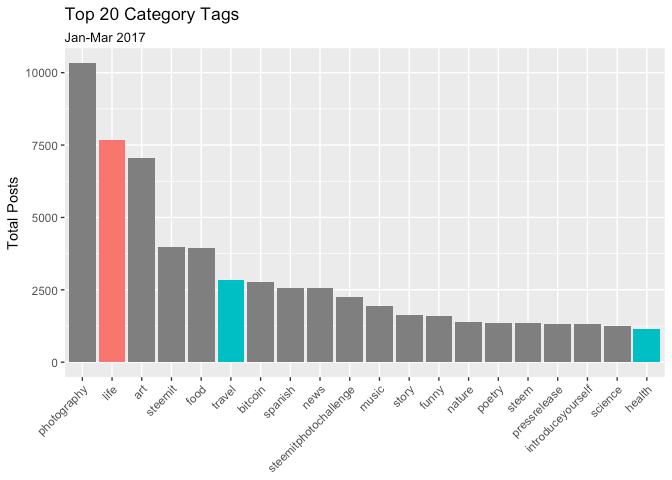
I drew data from January 2017 for the categories #Health and #Travel
  raw2<- mdb$find(query='{"created": {"$gte": {"$date": "2017-01-01T00:00:00.00Z"}, "$lte": {"$date": "2017-01-31T00:00:00.00Z"} },"category": {"$eq" : "health"} }', fields='{"_id":0, "body":1}')
  raw3<- mdb$find(query='{"created": {"$gte": {"$date": "2017-01-01T00:00:00.00Z"}, "$lte": {"$date": "2017-01-31T00:00:00.00Z"} },"category": {"$eq" : "travel"} }', fields='{"_id":0, "body":1}')
There isn't much data to work with.
- Life Category : 2432 Posts
- Health Category: 379 Posts
- Travel Category: 379 Posts
It appears that #Health and #Travel also contain a large number of URLs referring traffic out of the Steemit platforms. These are a similar mix of media hosts and CDNs.
Health Category Referral Destinations
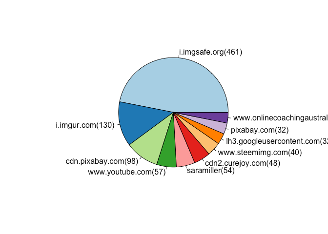
I can't explain the curious appearance of saramiller in this list.
Travel Category Referral Destinations
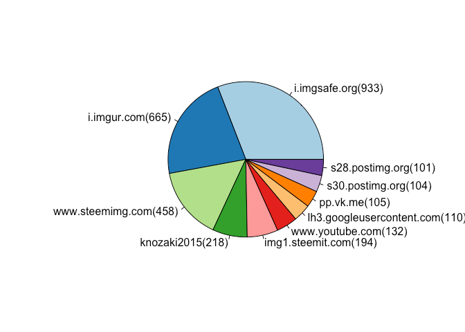
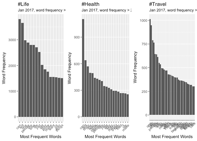
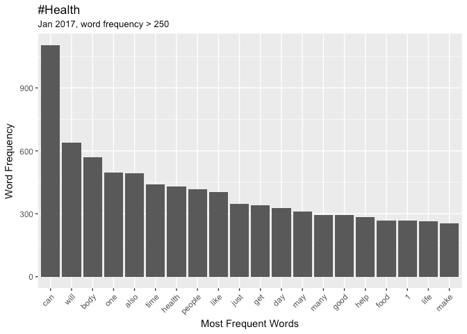
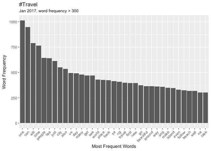
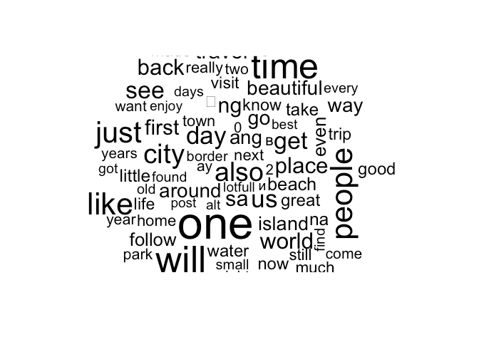
If we create a Corpus for Health and Travel and recalculate their Word Frequency we can compare them to the Life category.
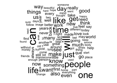
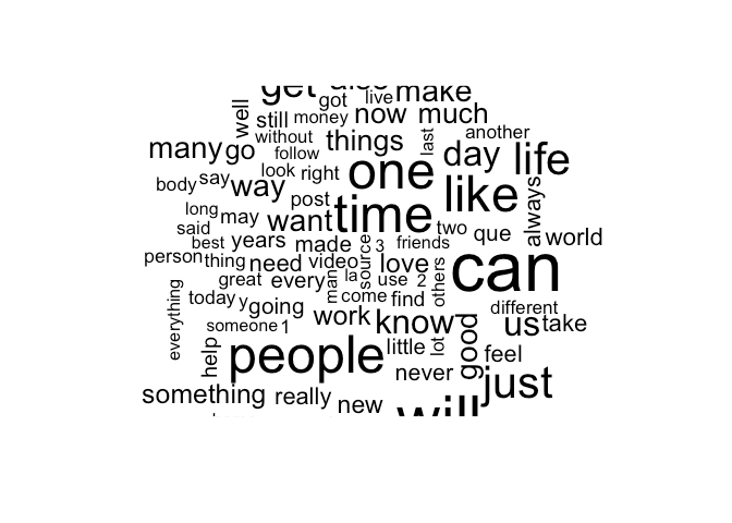
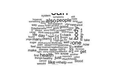
Given the significanty fewer posts in these categories I have to tune the Word Frequency parameters to observe the top performers. The Word Clouds, have a minimum frequency of 500.
Comparing Word Frequency
Health
Travel
Emoji & Emoticons
This is based on the very impressive work by Jessica Peterka-Bonetta. I won't repost her code or show how I butchered it so inelegantly. I also credit Tim Whitlock for his invaluable online resource.
Extracting and counting the Emojis in #Life, #Health and #Travel, show many similarities.
LIFE - Top Emoji for month of Jan 2017
| description | unicode | count | ||
|---|---|---|---|---|
| 1 | ⤴ | Arrow Curving | U+2934 | 37 |
| 2 | © | Copyright | U+00A9 | 31 |
| 3 | ♥ | Heart Suit | U+2665 | 23 |
| 4 | Ⓜ | Circled | U+24C2 | 9 |
| 5 | ™ | Trade Mark | U+2122 | 8 |
| 6 | ❤ | Red Heart | U+2764 | 3 |
| 7 | ® | Registered | U+00AE | 2 |
| 8 | ❄ | Snowflake | U+2744 | 2 |
| 9 | ✈ | Airplane | U+2708 | 1 |
| 10 | 😄 | Smiling Face | U+1F604 | 1 |
HEALTH - Top Emoji for month of Jan 2017
| description | unicode | count | ||
|---|---|---|---|---|
| 1 | © | Copyright | U+00A9 | 7 |
| 2 | ® | Registered | U+00AE | 5 |
| 3 | ❄ | Snowflake | U+2744 | 2 |
| 4 | ✌ | Victory Hand | U+270C | 2 |
| 5 | ♂ | Male Sign | U+2642 | 1 |
| 6 | ❤ | Red Heart | U+2764 | 1 |
| 7 | ☠ | Skull & Crossbones | U+2620 | 1 |
| 8 | ☀ | Sun | U+2600 | 1 |
TRAVEL - Top Emoji for month of Jan 2017
| description | unicode | count | ||
|---|---|---|---|---|
| 1 | © | Copyright | U+00A9 | 65 |
| 2 | ✈ | Airplane | U+2708 | 5 |
| 3 | ✔ | Heavy Check Mark | U+2714 | 2 |
| 4 | ⤴ | Arrow Curving | U+2934 | 2 |
| 5 | ® | Registered | U+00AE | 1 |
| 6 | ✌ | Victory Hand | U+270C | 1 |
I was somewhat surprised to see the "copyright", "registered" and "trade marked" emoji appearing so dominantly. For a community of open source advocates I'd expect a more liberal, re-sharing mindset. However this is a small sample size and there may be confounding factors such as user accounts belonging to commercial entities.
There are too few sentiment-emoji for sentiment analysis at this time. With a bigger dataset we can attempt to score sentiment with the weights defined by in the paper by P. Kralj Novak, J. Smailovic, B. Sluban & I. Mozetic.
CONSLUSIONS
The dataset is drawn from a period when Steem was les than one year old. It was unreasonable to expect more than light weight, trivial content from such an immature platform.
No obvious themes and topics could be discerned from the Tag Categories. This is a function of so little data. Rerunning this analysis later in 2018 may provide sufficient data to identify stronger word patterns and themes.
The common practice of cross-tagging, or tag-spamming will have confounding effects. As more data becomes available and tag use becomes more strategic on the part of the user, this situation will improve. However, given the incentive is up-voting rather than page ranking behavior will be slower to change.
I hope this analysis provides a framework to build on, with larger datasets in the future. Hopefully by then I'll have a better computer!
Posted on Utopian.io - Rewarding Open Source Contributors
Hey @morningtundra I am @utopian-io. I have just upvoted you!
Achievements
Community-Driven Witness!
I am the first and only Steem Community-Driven Witness. Participate on Discord. Lets GROW TOGETHER!
Up-vote this comment to grow my power and help Open Source contributions like this one. Want to chat? Join me on Discord https://discord.gg/Pc8HG9x
Would love to learn more about this, i'll check out the group.
.
@originalworks
Terrific analytics man, this is very useful information for people looking to target certain demos. Bravo -- subscribed!
I'm a lil smarter after reading this post. Thanks.
Thank you
Hopefully by then I'll have a better computer! :D -- I hope❤️
:-) You should see this piece of junk - on its 3rd battery, 2nd power supply, 2nd Screen and 2nd HDD. It's been dropped, splashed and frozen (in my car during a snow storm). It's a survivor for sure.
Thank You So Much For Sharing This As Well As Including The Links , Greatly Appreciated :)
You can gain more attention to your post, Just make it a little bit more attractive. Here is how can you do this !
https://steemit.com/steemit/@teamnepal/7-ways-make-your-post-get-real-attention
Great post, !
This is very interesting, I'd be interested to see what this analysis would look like if you only looked at posts over a certain reward amount, and filtered out auxiliary verbs like "can, will, would, should."
I see steemdata is nearly caught up. I might have another run at this in a few days after my surgery
I had a go at trying to answer this question https://utopian.io/utopian-io/@morningtundra/natural-language-text-analysis-of-most-up-voted-and-down-voted-posts-in-december-2017
thanks for sharing
I wonder how this would contrast if you did an analysis against Medium's content. Of course, Steemit is younger than Medium. I wonder when Steemit's content will reach the quality of Medium's posts. I wonder if that comparison is fair.
I hope with time it’ll get there as I’m getting rather tired of the spam and food pics. It feels like the early days of IGram.
Haha. Tired of those color contests, too.
Steemit on follow me back
HELLO FRIEND ... YOU ARE INCREDIBLE, THANK YOU FOR THIS DETAILED INFORMATION.BLESSINGS
oui bonne chose monsieur morningtundra
one who started early always has an advantage
Great post, I love how you outline your process.
As an aside, how large a portion of Steemit consists of Spanish or Korean speakers? I wonder if it's a big slice.
That’s a good questions I might try and answer in a future posts. I’d have to count posts containing espaniol. Counting other foreign character sets will be harder without help from native speakers. I can see from just eyeballing the data that nearly half use foreign character sets.
Thanks for answering, that answers my question. Not sure if that's useful information, though.
Thank You So Much Science To Share It And Including Links, Very Good :)
great post
Severo
we all are a strong family of steemit
Nice