Repository
https://github.com/scikit-learn/scikit-learn
What Will I Learn?
- Collect data from beem and SteemSQL
- 3D visualization of features
- Use different classifiers
- Compare classifiers accuracy
Requirements
- python
- basic concepts of data analysis / machine learning
Tools:
It looks like a lot of libraries, but it's a standard python toolset for data analysis / machine learning.

Difficulty
- Intermediate
Tutorial Contents
- Problem description
- Collecting data
- 3D visualization of features
- Overview and comparison of available classifiers
Problem description
The purpose of this tutorial is to build the account classifier (content creator vs scammer vs comment spammer vs bid-bot). In the previous part of this tutorial, we achieved an accuracy of 95%. And this is what the confusion matrix looks like:

The accuracy is quite good, but we will also check other available machine learning models. In one of the next parts of this series we will go on to build an API that will allow any Steem user to use this classifier.
Collecting data
The data was downloaded in a similar way to the previous part of the tutorial. Currently, each class has 769 records. The script that retrieves all the data can be found here.
The data looks as follows:
name followers followings follow ratio muters reputation effective sp own sp sp ratio curation_rewards posting_rewards witnesses_voted_for posts average_post_len comments average_comment_len comments_with_link_ratio posts_to_comments_ratio class
0 anthowarlike 212 34 0.160377 0 56.409193 1.349465e+02 134.946458 1.000000 0.654 265.146 0 0 0 0 0 0.000000 0.000000 0
1 gokcehan61 4117 16596 4.031091 19 51.233260 1.840426e+00 6.897189 0.266837 0.378 143.148 3 0 0 0 0 0.000000 0.000000 0
2 mimikombat 773 701 0.906856 2 60.575495 1.503410e+02 388.205087 0.387272 4.340 762.985 0 125 3366 401 50 0.084788 0.311721 0
3 stixxzyy 238 4 0.016807 0 55.103692 8.356541e+01 83.565407 1.000000 0.000 166.170 0 80 280 0 0 0.000000 0.000000 0
4 akintunde 2171 589 0.271304 9 62.343843 3.119804e+02 448.934538 0.694935 11.737 1025.171 19 21 1941 26 241 0.115385 0.807692 0
5 bryangav 718 80 0.111421 0 55.217102 2.791844e+02 77.046693 3.623574 3.779 183.609 8 62 3023 37 263 0.783784 1.675676 0
6 plouton 50 9 0.180000 0 44.422357 1.500954e+01 6.313641 2.377320 0.011 11.527 0 0 0 0 0 0.000000 0.000000 0
7 marzukie 1546 2585 1.672057 6 54.130093 9.463211e+01 94.632106 1.000000 2.988 146.743 30 77 2597 361 90 0.019391 0.213296 0
8 lisnabuah 25 2 0.080000 0 42.741003 1.190729e+01 0.269269 44.220849 0.002 5.931 0 0 0 0 0 0.000000 0.000000 0
9 nappingkid 255 15 0.058824 1 56.969551 1.773283e+02 177.328282 1.000000 1.110 274.575 0 103 290 8 45 0.000000 12.875000 0
10 itsmskali 118 24 0.203390 0 41.774677 5.015003e+00 3.569537 1.404945 0.022 4.982 0 0 0 0 0 0.000000 0.000000 0
11 rahmato 341 99 0.290323 0 34.397586 1.502713e+01 1.288114 11.665988 0.008 0.686 0 23 875 9 27 0.000000 2.555556 0
12 theuniqornaments 305 14 0.045902 0 45.984113 1.863325e+00 0.046184 40.345844 0.054 12.777 1 39 369 2 19 0.000000 19.500000 0
13 alexcarlos 232 25 0.107759 0 52.324648 4.336502e+01 43.365019 1.000000 0.064 83.009 0 50 1182 2 39 0.000000 25.000000 0
14 sharkhssn90 281 115 0.409253 0 26.253763 1.509236e+01 6.586708 2.291336 0.000 0.090 0 18 1106 25 121 0.000000 0.720000 0
15 omur61 976 1502 1.538934 1 56.939854 4.821556e+01 48.215558 1.000000 7.902 239.101 1 2 123 1 32 0.000000 2.000000 0
16 philberlin 141 50 0.354610 0 31.309064 1.500171e+01 3.211032 4.671927 0.007 0.305 0 0 0 0 0 0.000000 0.000000 0
17 chigz14 342 164 0.479532 2 56.755740 4.491221e+01 165.039345 0.272130 0.167 268.042 4 88 778 28 93 0.214286 3.142857 0
18 elysiian 1969 43 0.021838 7 60.425031 1.800332e+04 17074.531635 1.054396 291.260 1078.414 6 68 57 0 0 0.000000 0.000000 0
19 skizoweza 307 5 0.016287 53 59.502481 3.943580e+02 394.357979 1.000000 5.600 526.632 0 0 0 0 0 0.000000 0.000000 0
20 coretan 908 76 0.083700 4 61.023030 2.803443e+02 481.469079 0.582268 13.339 767.718 0 28 2257 49 83 0.040816 0.571429 0
21 tonygreene113 1329 265 0.199398 8 49.221399 2.278498e+02 227.849765 1.000000 4.193 77.221 7 48 911 570 128 0.629825 0.084211 0
22 tenpoundsterling 293 41 0.139932 0 51.745826 4.027079e+01 40.270792 1.000000 0.042 64.298 3 25 962 167 124 0.053892 0.149701 0
23 copypast3r 19 1 0.052632 0 25.000000 5.021256e+00 0.509150 9.862030 0.000 0.000 0 0 0 0 0 0.000000 0.000000 0
24 eae 859 428 0.498254 0 57.780078 1.530711e+02 153.071146 1.000000 1.217 327.817 0 107 1276 12 66 0.000000 8.916667 0
25 papyboys 330 99 0.300000 1 56.442663 2.003855e+01 120.254800 0.166634 0.046 239.335 1 116 1273 0 0 0.000000 0.000000 0
26 troonatnoor 409 144 0.352078 7 47.927954 4.434722e+01 44.347223 1.000000 0.000 18.675 0 16 3757 2 289 0.500000 8.000000 0
27 nowonline 544 324 0.595588 0 52.441200 1.474777e+02 147.477713 1.000000 0.679 75.321 0 24 6303 211 178 0.066351 0.113744 0
28 skizoweza 307 5 0.016287 53 59.502481 3.943580e+02 394.357979 1.000000 5.600 526.632 0 0 0 0 0 0.000000 0.000000 0
29 susanli3769 1321 288 0.218017 3 66.699240 5.969675e+03 3778.127511 1.580062 138.835 4059.769 9 93 2200 167 51 0.005988 0.556886 0
... ... ... ... ... ... ... ... ... ... ... ... ... ... ...
3D visualization of features
In the previous parts of this tutorial we have done 2D visualization, but equally well, we can do 3D visualization. We will use the mplot3d library and the code below.
# create 3D scatter plot
# x, y, z - names of features
def scatter_plot_3d(d, x, y, z):
    fig = plt.figure(figsize=(10, 10))
    # create 3D axes
    ax = Axes3D(fig)
    # plot points, cmap is colormap
    ax.scatter(d[x], d[y], d[z], c=d['class'], cmap=plt.cm.Accent, edgecolor='k', s=80)
    # set labels of each axis
    ax.set_xlabel(x)
    ax.set_ylabel(y)
    ax.set_zlabel(z)
    # add legend to plot
    # color of each legend label coresponds to color of given class
    ax.legend([label(color(150, 210, 150)), label(color(247, 192, 135)),
               label(color(235, 8, 144)), label(color(102, 102, 102))],
              ['content-creator', 'scammer', 'comment-spammer', 'bid-bot'], numpoints = 1)
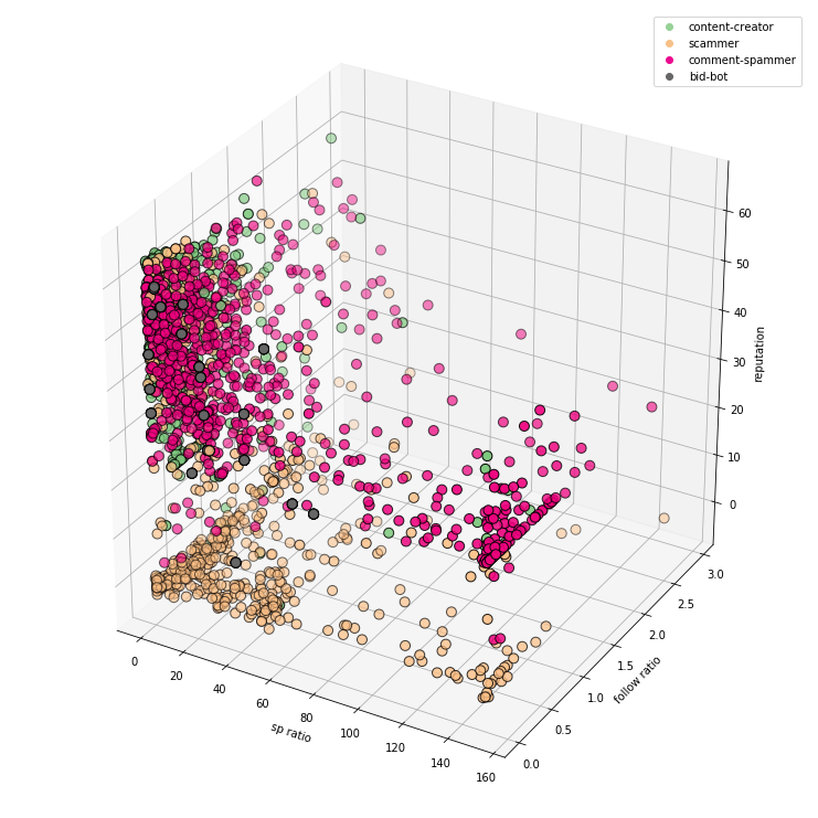
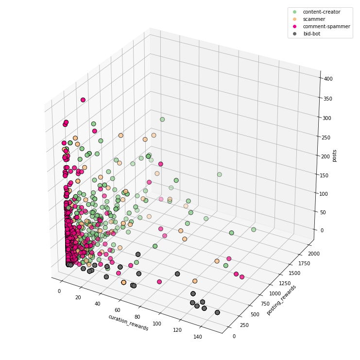
This allows you to place 3 features on the same chart at the same time.
followings + followers + muters:
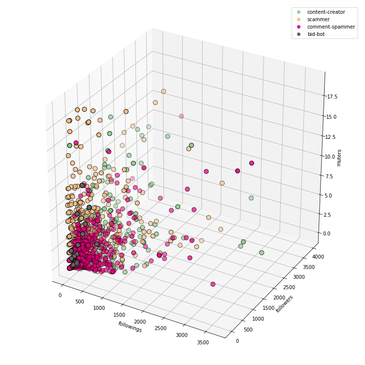
If we run the code as Jupyter Notebook, the charts are interactive.

sp ratio + follow ratio + reputation:
curation_rewards + posting_rewards + posts:
average_comment_len + comments_with_link_ratio + posts_to_comments_ratio:
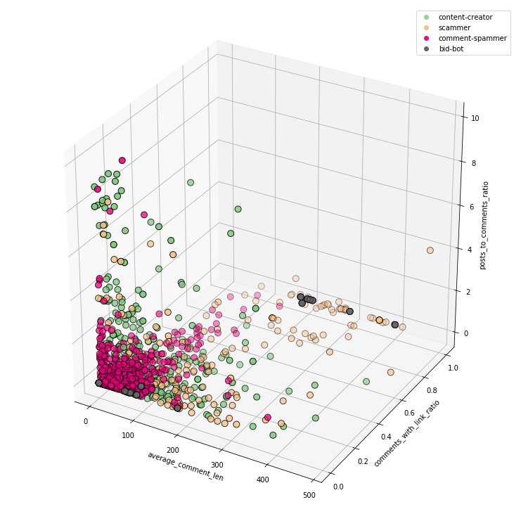
3D visualization has its advantages and disadvantages. We can put more information on one chart, but on the other hand, they are sometimes less readable.
Overview and comparison of available classifiers
Last time, we used classifiers like the neural network and the decision tree. The latter turned out to have better accuracy. But there are also many other classifiers that you can use:
- BernoulliNB - Naive Bayes classifier for multivariate Bernoulli models, is suitable for discrete data.
- GaussianNB - Gaussian Naive Bayes classifier
- KNeighborsClassifier - K-nearest neighbors classifier
- NearestCentroid - Nearest Centroid classifier, similiar to KNeighborsClassifier
- LinearSVC - Linear Support Vector Machine (SVM) classifier
In addition to accuracy and confusion matrices, we will also determine the execution time for each classifier.
X_cols = columns
y_cols = ['class']
X = df[X_cols]
y = df[y_cols]

# split data to training and test set
X_train, X_test, y_train, y_test = train_test_split(X, y, test_size=0.2, random_state=0)

# convert from pandas dataframe to plain array
y_train = np.array(y_train).ravel()
y_test = np.array(y_test).ravel()


classifiers = [
    ('DecisionTreeClassifier', DecisionTreeClassifier(max_depth=8)),
    ('BernoulliNB', BernoulliNB()),
    ('GaussianNB', GaussianNB()),
    ('KNeighborsClassifier', KNeighborsClassifier()),
    ('NearestCentroid', NearestCentroid()),
    ('LinearSVC', LinearSVC())]

# iterate over used classifiers
for clf_name, clf in classifiers:
    start = time.time()
    clf.fit(X_train, y_train) # train
    y_pred = clf.predict(X_test) # test
    end = time.time()
    print('%25s - accuracy: %.3f, execution time: %.3f ms' %
          (clf_name, accuracy_score(y_pred, y_test), end - start))
    cm = confusion_matrix(y_test, y_pred)
    plot_confusion_matrix(cm)
The results are as follows:
| Classifier | Accuracy | Execution time | Confusion matrix |
|---|---|---|---|
| DecisionTreeClassifier | 0.958 | 0.023 |  |
| BernoulliNB | 0.508 | 0.003 |  |
| GaussianNB | 0.360 | 0.003 |  |
| KNeighborsClassifier | 0.794 | 0.012 |  |
| NearestCentroid | 0.268 | 0.002 |  |
| LinearSVC | 0.656 | 0.933 |  |
The best result was obtained by the decision tree, which means that no better classifier was found for this problem. LinearSVC had a much longer execution time than other classifiers.
To visualize the decision tree, just use the following code:
import graphviz
from sklearn.tree import export_graphviz

# convert decition tree metadata to graph
graph = graphviz.Source(export_graphviz(
    classifiers[0][1],
    out_file=None,
    feature_names=X_cols,
    class_names=class_names,
    filled=True,
    rounded=True))

# set format of output file
graph.format = 'png'
# save graph to file
graph.render('DecisionTreeClassifier')

In the next part of the tutorial we will use Ensemble learning, i.e. using multiple machine learning algorithms to obtain better predictive performance.
Curriculum
- Machine learning (Keras) and Steem #1: User vs bid-bot binary classification
- Machine learning and Steem #2: Multiclass classification (content creator vs scammer vs comment spammer vs bid-bot)
- Machine learning and Steem #3: Account classification - accuracy improvement up to 95%
Conclusions
- the more data the better
- 3D visualization allows you to show more information than 2D visualization, but on the other hand, the data can be less readable
- it is worth to check the available classifiers, although sometimes the best results are obtained by the simplest ones
Hi @jacekw.dev! We are @steem-ua, a new Steem dApp, computing UserAuthority for all accounts on Steem. We are currently in test modus upvoting quality Utopian-io contributions! Nice work!
Nice!! I'm about to defend my master thesis which is all about ML and Scikit-learn :) Btw isn't SteemSQL paid service?
Thanks. Yes, SteemSQL is paid service, but definitely worth it, because at the moment it's the best database :)
Hey @jacekw.dev
Thanks for contributing on Utopian.
We’re already looking forward to your next contribution!
Want to chat? Join us on Discord https://discord.gg/h52nFrV.
Vote for Utopian Witness!
really cool. I have been looking at at way to use decision trees concepts ( entropy and information gain) on steemit data to calculate a user contribution score. Been working on it a while now.
I love the visualizations. Wish I had time to actually try out this tutorial. really appreciate your efforts here. Nice work
send you a dm on discord, hoping you will touch base with me
Congratulations @jacekw.dev! You have completed the following achievement on Steemit and have been rewarded with new badge(s) :
Click on the badge to view your Board of Honor.
If you no longer want to receive notifications, reply to this comment with the word
STOPCongratulations @jacekw.dev! You have completed the following achievement on Steemit and have been rewarded with new badge(s) :
Click on the badge to view your Board of Honor.
If you no longer want to receive notifications, reply to this comment with the word
STOPCongratulations @jacekw.dev! You have completed the following achievement on the Steem blockchain and have been rewarded with new badge(s) :
Click on the badge to view your Board of Honor.
If you no longer want to receive notifications, reply to this comment with the word
STOPDo not miss the last post from @steemitboard:
Congratulations @jacekw.dev! You have completed the following achievement on the Steem blockchain and have been rewarded with new badge(s) :
Click here to view your Board of Honor
If you no longer want to receive notifications, reply to this comment with the word
STOPDo not miss the last post from @steemitboard: