In my last post, I stated something rather paradoxical about solving non-homogeneous differential equations: ...to find a solution to the non-homogeneous equation, we need to find a solution to the non-homogeneous equation.
A bit of a 'Catch-22'? Well, in this post we'll walk through the first of such methods...

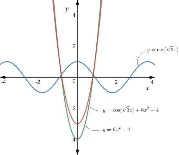
Figure 1. Graph of the particular solution to equation (6)
The method of undetermined coefficients is a simple, but effective way of finding solutions to the non-homogeneous equation. Here, we use more or less a trial-and-error approach to find solutions for  .
.
Rather than explaining how it's done, first let's just go through a few examples to understand the mechanics of finding these solutions. After that, we'll summarise the method. So let's go straight to Example 1...
Example 1
Let's find the particular solution to the equation (I started with the number (6), as it follows equation (5) from the last post)...

With initial conditions...

First, we must find the solution to the homogeneous equation...

...the characteristic equation of which is...

...giving rise to the roots...

...and thus the general solution to the homogeneous equation is...

Ok, so now that we have a solution to the homogeneous equation, we need to find a solution to the non-homogeneous equation.
How do we go about it?
Well, let's try a solution of the form that is similar to the term on the right-hand side of equation (6). Let's try...

...thus  and
and  . Let see how this goes when we substitute these expressions into (6)...

Now, equating the coefficients, we see that 3C = 18 (i.e. C = 6), but 2C = 0 as well (i.e. C = 0). This is a conflicting, or contradicting result.
So that obviously didn't work, but let's not give up here.
Let's try including some of the lower degrees to turn the trial solution into a polynomial...

Now, the first and second derivatives are...

..and...

And now substituting these into (6)...

So equating the coefficients again, we have...

...we also have...

...and finally, we have...

Therefore, our solution for  is...
is...

So, from (3) of the last post, the general solution is...

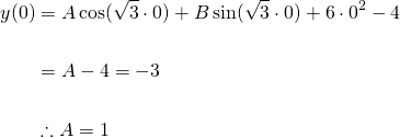
In similar fashion to previous methods of finding particular solutions, we apply the initial conditions. Firstly...

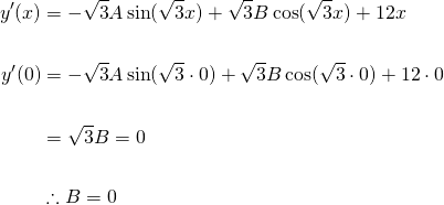
To apply the second initial condition, we need to find the first derivative...

And therefore, the final particular solution is...

Figure 1 above shows a graph of this solution. The solution is simply a superposition (i.e. a fancy way of saying 'addition') of an oscillating (circular) component:  ; and a polynomial component
  .
.
As you can see by the red curve, the solution is dominated by the polynomial.
We will go through another example in the next post.
Credits:
All equations in this tutorial were created with QuickLatex
First Order Differential Equations
- Introduction to Differential Equations - Part 1
- Differential Equations: Order and Linearity
- First-Order Differential Equations with Separable Variables - Example 1
- Separable Differential Equations - Example 2
- Modelling Exponential Growth of Bacteria with dy/dx = ky
- Modelling the Decay of Nuclear Medicine with dy/dx = -ky
- Exponential Decay: The mathematics behind your Camping Torch with dy/dx = -ky
- Mixing Salt & Water with Separable Differential Equations
- How Newton's Law of Cooling cools your Champagne
- The Logistic Model for Population Growth
- Predicting World Population Growth with the Logistic Model - Part 1
- Predicting World Population Growth with the Logistic Model - Part 2
- What's faster? Going up or Coming Down?
First order Non-linear Differential Equations
- There's a hole in my bucket! Let's turn it into a cool Math problem!
- The Calculus of Hot Chocolate Pouring!
- Foxes hunting Bunnies: Population Modelling with the Predator-Prey Equations
Second Order Differential Equations
- Introduction to Second Order Differential Equations
- Finding a Basis for solutions of Second Order ODE's
- Roots of Homogeneous Second Order ODE's and the Nature their Solutions
- Modelling with Second Order ODE's: Undamped Free Oscillations
- Modelling Car Suspension with ODE's: Damped Free Oscillations Part 1
- Modelling Car Suspension with ODE's: Damped Free Oscillations Part 2
- Modelling Car Suspension with ODE's: Damped Free Oscillations Part 3
- Non-homogeneous Differential Equations
- Solving Non-homogeneous ODE's: Method of Undetermined Coefficients Part 1
Please give me an Upvote and Resteem if you have found this tutorial helpful.
Feel free to ask me any math question by commenting below and I will try to help you in future posts.
Tip me some DogeCoin: A4f3URZSWDoJCkWhVttbR3RjGHRSuLpaP3
Tip me at PayPal: https://paypal.me/MasterWu
Welcome back again :o)
Thank you @mathowl! Once again, I'm going to try to be more consistent with my posting.
Congratulations @masterwu! You have completed the following achievement on the Steem blockchain and have been rewarded with new badge(s) :
Click here to view your Board of Honor
If you no longer want to receive notifications, reply to this comment with the word
STOPDo not miss the last post from @steemitboard:
This post has been voted on by the SteemSTEM curation team and voting trail in collaboration with @curie.
If you appreciate the work we are doing then consider voting both projects for witness by selecting stem.witness and curie!
For additional information please join us on the SteemSTEM discord and to get to know the rest of the community!