
In my last post, I detailed the results of using two popular machine learning techniques for learning how to aim artillery weapons in Arma 3. In this post I will describe in more detail how to set up your own machine learning pipeline for flexible data analysis, and give an example of how to set up a classifier and regressor with sample data.
Setting up the environment
Overview
This section will instruct you on how to:
- Install Anaconda3 5.1.0
- Install Visual Studio 2017 Community Edition
- Create a virtual environment for use in machine learning projects
- Add the virtual environment to Visual Studio
Getting Started
One step that can often be confusing when attempting to do any kind of machine learning (aside from actually learning how to interpret results from machine learning) in Python is setting up an environment where all the necessary tools are present and configured. To make this easier, I will detail step by step, line by line how to set up an environment and project to start doing meaningful machine learning.
These instructions will be provided for the 64-bit version of Windows 10.
Necessary Tools
You will first need to download and install the following programs:
- Anaconda3 5.1.0 (or later version)
- During installation it may ask you to check a box making Anaconda your default Python installation. Go ahead and check this box if you don't have Python already installed. Otherwise it is simply up to you if you want to make Anaconda your default Python.
- After installing Anaconda will prompt you to install Visual Studio Code. This is not the same as Visual Studio, and instead is a text editor. You can safely skip the installation for our purposes.
- Visual Studio 2017 Community Edition
- When installing I recommend checking the options for Python development. If you have already installed Anaconda then I don't recommend checking the option for Data science and analytical applications, as it will install an older version of Anaconda.
Anaconda is an extended version of Python with many packages for machine learning and data science included. It comes with its own package manager and environment creator that is easy to use. Installing Anaconda isn't strictly necessary for doing machine learning, but more likely than not you will end up installing many of the features included in Anaconda. Some packages, such as theano, are also much easier to install on Windows through Anaconda Navigator than via Python's default pip interface.
Visual Studio is useful for debugging code inline and giving somewhat intelligent autocomplete features while coding, saving you from having to look up every function in the packages we will be using. Again it isn't strictly necessary, but provides many useful features for doing work in programming. Visual Studio also makes it easy to select a virtual environment for your project, which I will explain in this post.
Creating a virtual environment with Anaconda Navigator
Why a virtual envrionment?
Virtual environments are useful tools for separating the execution environment of various projects. It gives you a nice way of controlling what packages are installed on a project-level, so if you end up working on projects that require different versions of the same package you do not run into issues.
Instructions
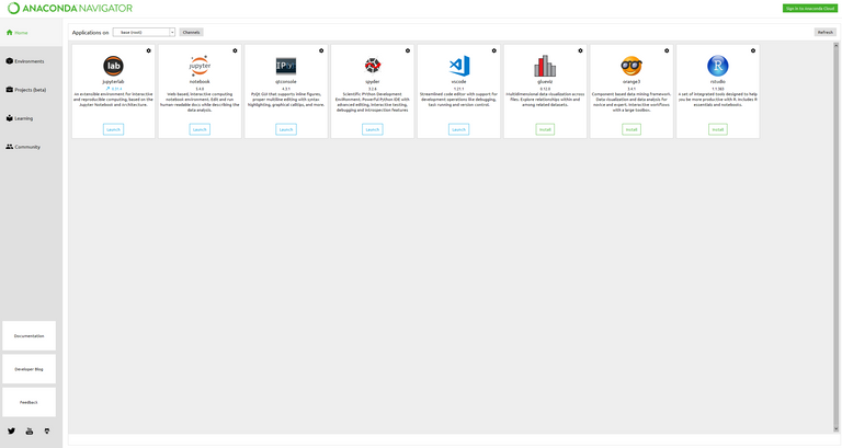
After you have installed the necessary tools, go ahead and open Anaconda Navigator. Navigator is an all-in-one interface for managing your Anaconda installation. Once Navigator loads, you should be greeted with a home page that looks something like this:
The default Anaconda Navigator Home Page
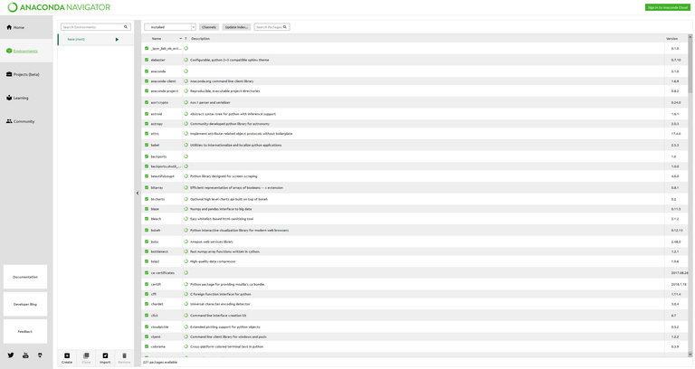
Click on the "Environments" tab on the left to see this page:
The default Anaconda Navigator Environments Page
Near the bottom of the environments page, click the "Create" button and enter a name for the new environment. Since we will want to use this environment as a base for machine learning projects, I suggest a name such as "machine_learning". Once we have configured the environment, we can clone it and modify the clone for each individual project we do.
It may take a minute for Anaconda Navigator to create the new virtual environment. Wait for it to finish before proceeding.
Installing required packages for machine learning in Python
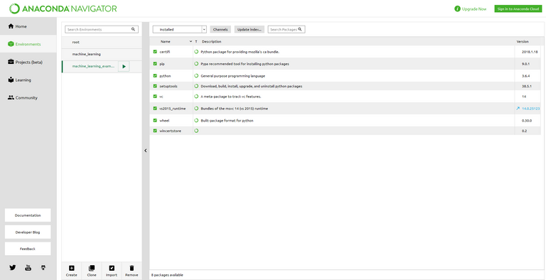
Once the new environment is created, you should see two items in the environments list on the left side of the Environments tab. Select the new environment to see which Python packages are installed. If creating the new environment completed successfully, you should see something like the image below:
The base virtual environment created by Anaconda Navigator
You should see only a few packages installed to the environment, such as pip, python, setuptools etc.
You can install new packages by entering the name of the package we need in the "Search Packages" input field and selecting the "Not Installed" option in the dropdown at the top of the list of packages on the right side of the screen. Once you find the package you would like to install, select the check box to the left of the package name and click the green "Apply" button in the bottom right corner.
Here are the packages I recommend installing for a basic machine learning workflow (for non-neural network projects):
- scikit-learn
- scipy
- numpy
- pandas
- matplotlib
Scikit-learn includes many helpful libraries for data preprocessing, machine learning models, and model evaulation. You can even create pipelines that do all the necessary operations to data, train a model, and evaluate its performance for multiple hyperparameter settings.
Scipy includes some helpful features for mathematical functions, such as calculating the spatial distance between points and other types of data calculations.
Numpy is an extremely powerful library for performing computationally intense mathematical functions for transforming data.
Pandas is a helpful library for reading, writing, and organizing data in your machine learning workflow.
Matplotlib is an easy to use tool for visualizing parts of your data to help you gain an intuitive understanding of it, which can greatly assist your selection, tuning, and evaluation of the performance of a machine learning model.
Configuring Visual Studio to use the Anaconda virtual environment
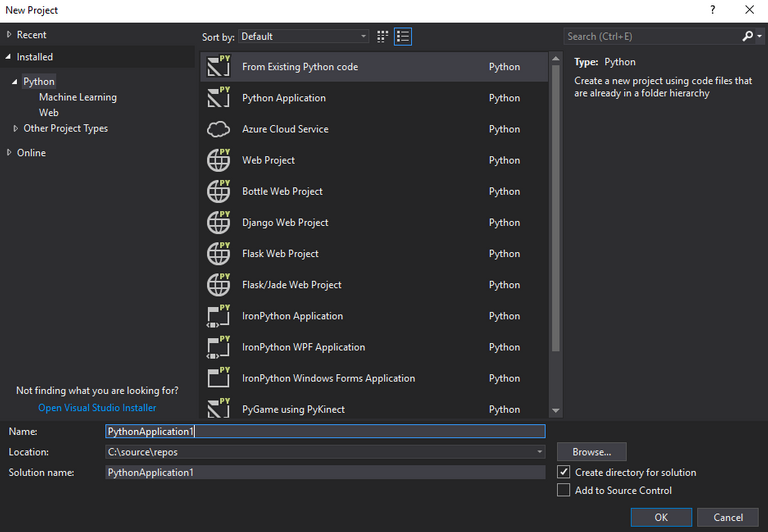
Open Visual Studio and click File>New Project. Select the "Python" section on the left side of the window that opens and select "Python Application" from the list in the center of the window.
The new project window
You can assign any name you like to the project. Once you choose a name and location for the project, go ahead and ensure that both check boxes for "Create directory for solution" and "Add to Source Control" are checked. Then click the OK button to create the Visual Studio project.
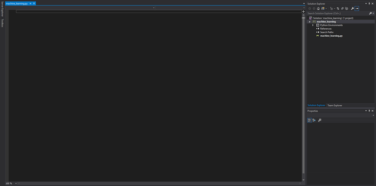
After a moment, you will be presented with an empty python file bearing the name of the project, and a menu on the right detailing the files in the project (the "Solution Explorer").
You should see something like this after creating a new project
Expand the "Python Environments" section of the solution explorer to see the currently selected Python interpreter for the project. By default the Python environment will be the default installation of Python on your machine. If you installed Anaconda as your default Python installation, than it will include all of the default Anaconda packages.
While it is possible to skip the virtual environment step and just start coding if Anaconda is the default installation on your machine, it is good practice to isolate your projects with virtual environments and generate requirements.txt files so other people with different setups can easily download and run your code.
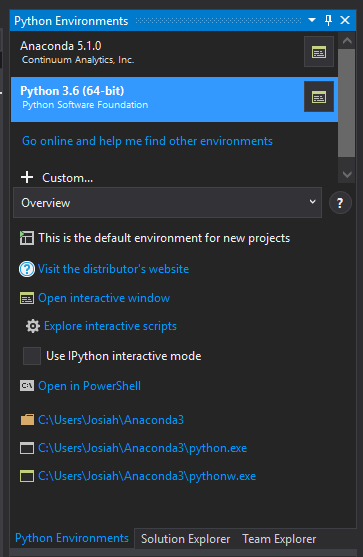
To add the virtual environment we created in Anaconda Navigator to our project in Visual Studio, right click the "Python Environments" section of the Solution Explorer and click "View All Python Environments". This will open the "Python Environments" window in the right panel.
The Python Environments Window
Click the "+" button labeled "Cusom..." and give it the same name as the environment you created in Anaconda Navigator in the "Description" field.
After giving the environment a name, click the "..." button next to the "Prefix path" field and browse to the root folder of the environment created by Anaconda Navigator. You can find where the environment is located by hovering your mouse over the environment in Navigator. By default Anaconda Navaigator will place environments in your C:\Users\username\Anaconda3\envs folder. Once you find the folder that matches the name of the environment you are trying to add, click the "Select Folder" button in the file explorer to select it as the containing folder for Visual Studio to use.
Once you have selected the "Prefix path" folder, click "Auto Detect" to fill in the remaining fields. If auto detect fails to fill in the rest of the fields, double check that your supplied prefix path matches the location of the environment given by Anaconda Navigator.
After the rest of the fields are filled in, click the "Apply" button to add the Anaconda Python environment to Visual Studio. This will add the environment to the list presented in the "Python Environments" window in the right panel.
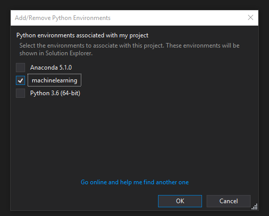
Close the "Python Environments" window to return to the Solution Explorer, then right click on the "Python Environments" section in the Solution Explorer. Click "Add/Remove Python Environments" and ensure that only the environment that matches the name from the Anaconda Navigator environment we created is checked. Then click ok.
Make sure only the environment we made in Anaconda Navigator is checked.
After a short moment, Visual Studio will be configured to use the environment that we created in Navigator. You can verify that the environment is correct by expanding the environment in the Solution Explorer and comparing the installed packages with what is displayed in the Anaconda Navigator package list for the environment.
Finally, do a quick check to make sure all the packages we need are installed. Add the following lines to the blank python file in the project:
import sklearn
import scipy
import numpy
import pandas
import matplotlib

print('All packages loaded successfully')
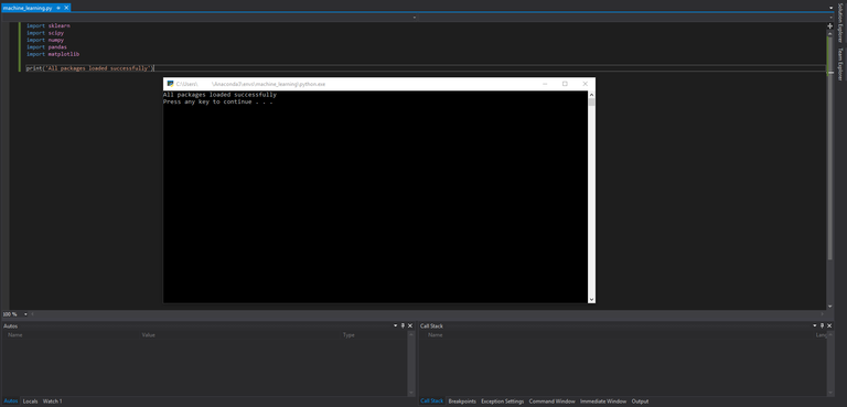
Click the green arrow at the top of the Visual Studio interface with the text "Attach..." label and observe the output of your program.
If everything is configured correctly, you should see the following output:
If you see this you are ready to start programming!
If you've followed this far then congratulations, most of the annoying setup phase is done! Take a five-minute coffee or water break and come back once you are ready, I'll wait for you.
Building a Machine Learning Dataflow in Python
For this tutorial, we will:
- Read data from a .csv file into our program
- Visualize the input data to gain intuition for model selection
- Split our data into training and testing sets
- Feed our training data into a pipeline which will:
- Standardize our data
- Train a classifier and regressor on the training data
- Evaluate the different hyperparameters to give us the best model
- Test our model against the test data set
- Visualize the model
Reading data for machine learning
For this example, we will use a dataset that consists of nearly 300 datapoints. Our example data will conform to the function f(x, y) = sin(x) + cos(y) + rand() * .1, with the additional category specifying if the result is positive or negative. This is the so called "true function" that we want our machine learning algorithm to learn to approximate. Our true function includes some randomness since most data in the wild does not perfectly conform to a mathematical function. You can download this example data here.
The example data follows the form:
| x | y | z | category |
|---|---|---|---|
| 2.449547331 | 2.449982339 | -0.1321066942 | neg |
| 0.8890124106 | 4.253728699 | 0.3337025175 | pos |
| 2.627823955 | 0.3270213974 | 1.438466224 | pos |
| ... | ... | ... | ... |
To read the data into our program, we will use the follwing code:
import pandas as pd

# The location of the data file
path = 'example_data.csv'
# Create a dataframe to hold the data from the csv
df = pd.read_csv(path)
# One-hot encode labels
df = pd.get_dummies(df)
This will take a string path, such as example_data.csv and create a pandas dataframe to hold the data. In this example, the example_data.csv file is in the same file as the machine_learning.py file created by Visual Studio.
After we get the dataframe, you can call get_dummies to do what is called One-hot encoding. One-hot encoding transforms categorical data (such as our pos and neg labels) into columns with a numerical value indicating which category was used (a 1 in the pos category means that it had a category value of pos). This gives our learning algorithm a nice way of understanding categorical data without making mistakes in thinking that neg is bigger than pos and the like.
Now that you have read the csv data into a pandas Dataframe object, you can access the columns by simply using the name of the column you want to access and the row by its position in the table:
>>> df['x']
<Series, len() = 300>
>>> df['y']
<Series, len() = 300>
>>> df['x'][0]
1.811662492
>>> df['z'][:5]
0    0.069672
1    0.836167
2    1.730618
3    0.925830
4    0.230684
Name: z, dtype: float64
Example usages of a pandas dataframe created from our example data. For more information on using pandas dataframes, please visit their documentation on their website
Visualizing the dataset
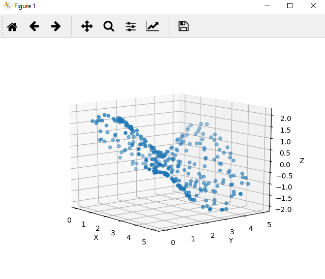
Before you embark on selecting a machine learning model, it's usually a good idea to do some exploration of the data you want to use. To do that, we will make some plots to gain insight into how the data might be structured. Even though for this example we already know the structure of the data, most problems do not have a neat mathematical formulation behind them.
We can attempt to visualize the data with the following code:
import matplotlib.pyplot as plt
from mpl_toolkits.mplot3d import Axes3D

# Create a 3d scatter plot of the data
fig = plt.figure()
ax = fig.add_subplot(111, projection='3d')

ax.scatter(df['x'], df['y'], df['z'])
ax.set_xlabel('X')
ax.set_ylabel('Y')
ax.set_zlabel('Z')

plt.show()
Values seem to move smoothly in both the x and y axes
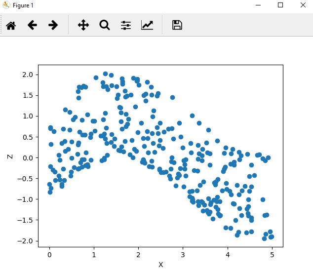
# Create a 2d scatter plot of X vs. Z
fig = plt.figure()
ax = fig.add_subplot(111)

ax.scatter(df['x'], df['z'])
ax.set_xlabel('X')
ax.set_ylabel('Z')

plt.show()
This plot shows a clear smooth relationship between our inputs and our outpus, and suggests that the underlying structure is simple.
This small example demonstrates the usefulness in visualizing a dataset with just a few dimensions. Often datasets have many more dimensions, which make visualization a challenging and intensive task. However, our exploration of the data has revealed that Z values move smoothly across our inputs.
These properties give you a hint that you might be working with a trigonometric function, which have the additional properties of being continuous and cyclical functions.
Creating training and testing data
Now that you have your data in a neatly organized pandas dataframe and have explored the data a bit, you need to split it into training and testing data. The rationale for this division is that you should try to pick a model that performs well against data you haven't seen. This is because some models overfit the data used to train it, and despite performing well on the training data, can peform very poorly on new data. Our test dataset gives you an idea of how much your model might be suffering from overfitting.
To split your data into two segments for training and testing, you can use the handy scikit-learn function, train_test_split:
from sklearn.model_selection import train_test_split

# We will train the model to predict Z and the category of the data from the X and Y values

# Create empty Dataframes
X = pd.DataFrame()
Y = pd.DataFrame()

# Add data input data to the X Dataframe
X['x'] = df['x']
X['y'] = df['y']

# Add label data to the Y Dataframe
# Because we one-hot encoded, loop over column names and add the columns not used in the X Dataframe
for col in df.columns.values:
    if col not in ['x', 'y']:
        Y[col] = df[col]

# Create separate datasets for training and testing
x_train, x_test, y_train, y_test = train_test_split(X, Y, test_size=0.3)
This block of code will move the input data to the machine learning algorithm into the X dataframe, and the correct labels to use for training into the Y dataframe. Then it will split these two dataframes into training and test sets, and the amount used for testing is defined in the test_size input to the test_train_split function, which represents the percentage of data to allocate to the test set.
For a basic sanity check, you can output the values of the training and testing sets:
>>> x_train
<DataFrame, len() = 210>
>>> x_test
<DataFrame, len() = 90>
>>> print(x_train)
            x         y
73   1.273996  0.806593
215  2.478684  2.980329
135  3.887038  4.554521
...
>>> print(y_train)
            z  category_neg  category_pos
73   1.706939             0             1
215 -0.290810             1             0
135 -0.794101             1             0
...
As you can see, x_train only has the columns "x" and "y", whereas y_train only has the columns z, category_neg, and category_pos. Also the values in each column seem to be correct, as the x and y columns have positive integers, and the z, category_neg, and category_pos columns have float values between -2 and 2 and a value of pos or neg respectively.
Selecting a model for fitting
There are many possible models we could choose from to attempt to fit this data. A comprehensive list and analysis of all the possible models we could choose is well beyond the scope of this post, but here are a list of popular non-neural network approaches (neural networks will be covered in a separate post):
A notable distinction between these models and neural networks is that in these models the decision process tends to be easier to interpret.
For this example, we will select a logistic regression approach for classification, and a linear regressor for regression. While logistic regression may not be as powerful as support vector machines, it has the very important advantage in being much easier to train, allowing us to find the right hyperparameters much more quickly than if we tried to use a support vector machine. For the same reason, we also choose the linear regressor over a support vector regressor.
From our exploration of the data, we noticed that it seems to follow a very smooth pattern that could be well approximated by a polynomial. For this reason we will apply polynomial feature fitting to our data before sending it to our learning algorithms. This is because the non-linearity of the data will make our two linear models (Logisitic Regression is still a linear classifier) perform poorly in non-transformed settings. By applying polynomial feature fitting, we move the linear model into a setting where the data looks more linear.
If these justifications are difficult to follow, don't worry. Understanding the uses of different classifiers and regressors and transforming the data to maximize the strengths of those models is a large part of what data scientists study to improve their craft.
Creating a pipeline to train the model
With few exceptions, data needs to be "brought on the same scale" before it is given to a machine learning model. This is because high numerical values in one dimension can overpower small values in another, and thus the model becomes trained to prioritize the high-value dimensions--even if they aren't more important than the small value dimensions. Putting the dimensions on an even playing field will greatly improve the accuracy of the model.
It should be noted that decision trees are not susceptible to this problem, and data can be fed "as-is" to either a single decision tree or random forest.
Standardization vs. Unit Vectorization
When it comes to scaling our data, there are two popular choices, standardization and unit vectorization. Standardization redefines each data value relative to all the other data points based on how "rare" the data point is. Unit vectorization compresses the range of all data points onto the same scale.
Standardization has the advantage that outliers do not compress the scale of the rest of the data, so for this case we will choose standardization. Our z data is also already neatly confined, so additional compression of the range of data will likely yield little benefit.
Initializing the Pipeline
A handy feature of the sklearn library is its inclusion of a Pipline, which is a structure for performing data preprocessing, model training, and model evaluation on the training data. Use of a Pipeline is not strictly necessary, but it is handy for organizing all of the steps involved in creating a model.
An important aspect of this problem to note is that we have two separate types of problems to solve, one is a classification problem, whether the inputs produce a positive or negative value, and the other is a regression problem, the value of z from the given x and y values.
To create our pipeline, we can use the following code:
from sklearn.pipeline import Pipeline
from sklearn.preprocessing import StandardScaler
from sklearn.preprocessing import PolynomialFeatures
from sklearn.linear_model import LinearRegression
from sklearn.linear_model import LogisticRegression

# Create pipelines for training machine learning models
# The pipeline for the classification aspect of the problem
pipe_clf = Pipeline([('scl', StandardScaler()),
                     ('poly', PolynomialFeatures()),
                     ('clf', LogisticRegression())])
# The pipeline for the regression aspect of the problem
pipe_regr = Pipeline([('scl', StandardScaler()),
                      ('poly', PolynomialFeatures()),
                      ('linear', LinearRegression(fit_intercept=False))])
This will create two pipelines, one to handle the classification task, and the other to handle regression. You will also need to think about how to tune the hyperparameters of these two models, such as the C and tolerance values for logistic regression and the degree for the polynomial transformation. Luckily, you don't have to do this by hand.
Hyperparameter Tuning
If your dataset is small enough, you can run a grid search over a range of defined hyperparameters and get the model that performs the best. A grid search will exhaustively cover all options you supply though, so it may take too long to complete depending on the size of your data.
An approach that works better for larger datasets is called a randomized search. A randomized search takes a range of possible hyperparameters and samples the range distribution instead of trying each value exhaustively. This can be much faster than a grid search, but may also miss certain combinations of hyperparameters that yield good results. For this example we will use a randomized search since most machine learning applications use large datasets.
Scikit-learn includes a randomized searcher named RandomizedSearchCV which we can use to tune the models.
We can create our random searches via the following code:
from sklearn.model_selection import RandomizedSearchCV
from scipy.stats import expon
from scipy.stats import randint

# Create the randomized searches
c_range_clf = expon(scale=1)
tol_range = expon(scale=1e-4)
degree_range = randint(1, 10)

# Define the parameter distribution for the classifier
param_dist_clf = {'poly__degree': degree_range,
                  'clf__C': c_range_clf,
                  'clf__tol': tol_range,
                  'clf__solver': ['newton-cg', 'lbfgs', 'liblinear']}

# Define the parameter distribution for the regressor
param_dist_regr = {'poly__degree': degree_range}

# Initialize the randomized search classifier
rs_clf = RandomizedSearchCV(pipe_clf,
                            param_dist_clf,
                            n_iter=300,
                            scoring='accuracy',
                            cv=10,
                            n_jobs=-1,
                            verbose=1)

# Initialize the randomized search regressor
rs_regr = RandomizedSearchCV(pipe_regr,
                            param_dist_regr,
                            n_iter=50,
                            scoring='r2',
                            cv=10,
                            n_jobs=-1,
                            verbose=1)

# Split the test and training labels for classification and regression
y_train_clf = pd.DataFrame()
y_test_clf = pd.DataFrame()

y_train_regr = pd.DataFrame()
y_test_regr = pd.DataFrame()

for col in y_train.columns.values:
    if 'z' in col:
        # Create regression labels
        y_train_regr[col] = y_train[col]
        y_test_regr[col] = y_test[col]
    else:
        # Create classification labels
        y_train_clf[col] = y_train[col]
        y_test_clf[col] = y_test[col]
Randomized search parameters
The n_iter parameter defines how many samples will be taken from the hyperparameter space you supply, so in general a higher value means it will try more models. This can improve accuracy but also lengthens training time. Feel free to adjust the n_iter parameter to a value that suits the capabilities of your machine.
The n_jobs parameter defines how many cores your computer will use to search the hyperparameter space. A value of -1 allows the program to use all available cores, and a positive number greater than one will specify how many cores to use. If you decide to use more than one core, ensure that all of your code follows a simple check:
if __name__ == '__main__':
    # Put all of your code indented under here
to prevent the newly spawned threads from starting everything over.
The cv parameter determines how much cross validation to perform on each model. The higher the value, the more tests it will perform on each model. The total number of tested models will be equal to cv * n_iter so you should adjust the cv, n_iter, and n_jobs parameters based on the capabilities of your machine.
The scoring parameter defines which metric will be used to evaulate the explored models. I selected accuracy for the classifier, since you can easily grade how many points are correctly classified. For the regressor, I chose r2 since you want the regressor to produce values close--but perhaps not exactly--to the test values. If we chose accuracy for the regressor, it would be very difficult for the randomized searcher to compare models since they would all have very low scores.
Handling multiple outputs
Since the classifier needs to produce multiple outputs (a value for both the category_pos and category_neg columns), you need to add an extra step after defining rs_clf. By default the LogisticRegression class in sklearn only produces one output; to make it produce multiple outputs you need to leverage the MultiOutputClassifier from sklearn.multioutput.
The following code will ensure that the classifier can handle having to produce two outputs:
from sklearn.multioutput import MultiOutputClassifier

mo_clf = MultiOutputClassifier(rs_clf)
This will train a model for each output required.
Fitting the data
Now that the classifier and regressor pipelines are both initialized and configured, it's time to fit the models to the data. This can be achieved in just two lines of code:
mo_clf.fit(x_train, y_train_clf)
rs_regr.fit(x_train, y_train_regr)
Executing these lines of code may take several minutes depending on the parameters given to the randomized searchers and the capabilities of your machine.
Evaluating the models
Once the model has been fit, it's time to see how well it performs on data it has not seen. You can quickly test the models by asking them to make predictions on our test data, which was created at the same time as the training data. Calling the score method of the models will compare the predicted results from the model with the actual results from the test data:
# Print the results of the fit on the test data
print('Test classification score: %.3f' % mo_clf.score(x_test, y_test_clf))
print('Test regression R2 score: %.3f' % rs_regr.score(x_test, y_test_regr))
After fitting the models, you should expect to see results similar to the ones below:
>>> Test classification score: 0.922
>>> Test regression R2 score: 0.999
These results seem promising, with a 92.2% accuracy score for the classifier and a nearly perfect score for the regressor. To better understand the differences in scores it helps to visualize the decision surface of the models.
Visualizing Decision Surfaces
To understand how the models are making decisions, you can plot the decision surfaces of each model to see how the model might be over or underfitting and hone the hyperparameter tuning in the configuration for the randomized search.
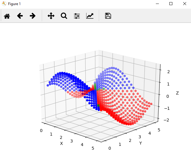
To do this, you can simply plot predicted outputs over a range of given inputs and compare that with the test data. For instance, take a look at the output from the X vs. Z plot of the regressor produced by the following code:
import numpy as np

# Plot the decision surfaces of the classifier and regressor
x = pd.DataFrame(np.linspace(0, 5, 25))
y = pd.DataFrame(np.linspace(0, 5, 25))

# Create a grid to plot our predicted values over
surf_x = pd.DataFrame(np.array(np.meshgrid(x, y, )).T.reshape(-1, 2))
surf_z = pd.DataFrame()

# Predict a value for each (x, y) pair in the grid
surf_z['z'] = [x[0] for x in rs_regr.predict(surf_x).tolist()]

# Translate our one-hot encoded labels back into a single list of string values
category_list = []
for x in mo_clf.predict(surf_x).tolist():
    if x[0] == 0 and x[1] == 1:
        category_list += ['pos']
    elif x[0] == 1 and x[1] == 0:
        category_list += ['neg']
    else:
        category_list += ['unk']

surf_z['cat'] = category_list

# Separate our values into separate surfaces so we can easily color the different categories from the classifier
pos_surf = surf_z.copy()
neg_surf = surf_z.copy()
unk_surf = surf_z.copy()

# Fill in values that don't match the label with NaN
pos_surf[pos_surf['cat'] != 'pos'] = np.nan
neg_surf[neg_surf['cat'] != 'neg'] = np.nan
unk_surf[unk_surf['cat'] != 'unk'] = np.nan

# Make the plot
fig = plt.figure()
ax = fig.add_subplot(111, projection='3d')
ax.scatter(surf_x[0], surf_x[1], pos_surf['z'], color='b')
ax.scatter(surf_x[0], surf_x[1], neg_surf['z'], color='r')
ax.scatter(surf_x[0], surf_x[1], unk_surf['z'], color='g')
ax.set_xlabel('X')
ax.set_ylabel('Y')
ax.set_zlabel('Z')

plt.show()
If you've properly used the code above, you should see a graph that resembles the following:
Each point plotted is a prediction from the regressor model. A blue color indicates that our classifier believes the value to be positive, a red color indicates that our classifier believes the value to be negative, and a green color means the classifier can't tell.
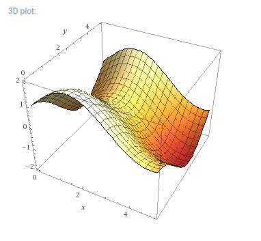
It's clear that the classifier has some trouble with inputs that have results near zero, but the shape of the model looks very close to the shape of the training and test data. For comparison, here is the actual solution space for f(x, y) = sin(x) + cos(y):
The true function space, without added randomness. Courtesy of WolframAlpha
If the decision surface looked strange, you could go back and change the configuration of the randomized searchers, swap out different models for fitting, or try different transformations of the data with minimal changes to this code base.
Summary
In this post you learned how to:
- Setup an environment for machine learning in Windows with Anaconda and Visual Studio
- Read a csv file into a pandas dataframe
- Explore the data using matplotlib
- Create a pipeline for data preprocessing and model fitting using sklearn
- Fit a machine learning model to the read data
- Evaluate the performance of a machine learning model
- Visualize the decision surface of a generated model
I've tried to be as comprehensive as possible without going into full depth in each of the mentioned topics, but if I missed something please feel free to ask a question in the comments below.
Congratulations! Your post has been selected as a daily Steemit truffle! It is listed on rank 7 of all contributions awarded today. You can find the TOP DAILY TRUFFLE PICKS HERE.
I upvoted your contribution because to my mind your post is at least 17 SBD worth and should receive 86 votes. It's now up to the lovely Steemit community to make this come true.
I am
TrufflePig, an Artificial Intelligence Bot that helps minnows and content curators using Machine Learning. If you are curious how I select content, you can find an explanation here!Have a nice day and sincerely yours,

TrufflePigMy only issue with this post is the first image. Even if you found it on pixabay you should still list the source of it. But otherwise, I think your post is good.
Got it, I'll post the source with it.
Congratulations @chosunone! You received a personal award!
Click here to view your Board
Congratulations @chosunone! You received a personal award!
You can view your badges on your Steem Board and compare to others on the Steem Ranking
Vote for @Steemitboard as a witness to get one more award and increased upvotes!