
Cryptography and randomness are interlinked on a fundamental level. When we encrypt a secret we want that result to look like completely random gibberish. In fact, if an external observer manages to notice any non-random patterns in our encrypted secret, that would be something they can exploit in order to recover parts of our secret. If you imagine cryptography as a ‘factory’, then for it to work well it has to be constantly lubricated by a fair amount of random entropy, otherwise the complicated machinery will explode in a spectacular fashion.
While that makes modern cryptography strong, it is very hard to find sources of good randomness. In fact, mathematicians have proven that if somebody gives you a seemingly random string, you cannot by any means ever prove if it is truly random (i.e. unpredictably generated), or if it just appears random, e.g. an adversary who wants to steal your secrets just crafted that string to look random. Since you cannot verifiably test any external service for the quality of its “true randomness”, in order to create a secure system you have to procure your own. Scientists have understood for a long time that it is pointless trying to hide the details of cryptographic algorithms, and they are widely known to everybody, including hostile attackers. The only things attackers do not know is the entropy of your cryptosystem — each bit of good (i.e. truly unpredictable) entropy creates a bit of cryptographic strength that protects your secrets.
Because cryptography requires a lot of unpredictable randomness, scientists have found many sources of “true” entropy — natural processes that through the laws of physics or chemistry constantly produce highly unpredictable, random results. Unfortunately, all these sources are inconvenient to use, because they require special purpose hardware or even more cumbersome setups. Current state of the art cryptography allows taking small, unpredictable seeds of randomness from the physical world, and spinning them up into endless, unpredictable, random streams of data. Modern computers and phones are equipped with highly sophisticated systems that do just that, so in general you can always use your computer’s /dev/urandom device when you need an unlimited source of randomness. If you are reading this on your MacBook right now, you can type the following command into the Terminal app to get as many random strings as you need: cat /dev/urandom | head -c 32 | base64 (substitute 32 to get longer or shorter strings).
One of the applications for natural entropy sources is building secure cryptosystems hosted on “cloud” servers. In such cases, we no longer have physical computers under our full control. There are a few ways to feed entropy into virtual computers, yet they all bear the same weakness cryptographers hate most of all — it requires blind trust of an external party to do the “right thing”. This is not optimal. Even the most respected cloud providers are still run by human beings who are known to make mistakes from time to time. Cryptographers prefer to be protected not by well-meaning humans, but by fundamental mathematical laws. And even the best corporations can be penetrated by hackers and hostile governments. As a customer of cloud services, there are simply no tests you can do to verify that your virtual host is getting “good” randomness from your trusted provider, or “bad” randomness that is subverted by hackers — they would look exactly the same. In fact, it will be enough for hackers to just make a copy of real, “true” randomness generated by the host hardware: it still will be perfect randomness received by your system, yet at same time it will be fully predictable (since the hackers would see it before you do). One popular version of Linux even created new service to help “pollinate” virtual machines with external randomness when they boot up.
In this article, we are going to show you how to create a new source of “true” thermal entropy from any Apple iOS device that is verifiably under your own control that nobody else can intercept or spoof. Having an independent, extra source of “true” entropy is useful because entropy failures are very hard to detect — there is no “flashing red light” to alert us when our main source of entropy fails for any reason. When used with reasonable precautions multiple sources of natural, “true” entropy allows us to build stronger cryptosystems.
A Noisy Phone
One of our open source products is the Zax relay which allows for asynchronous, anonymous and encrypted process-to-process communications between different devices, which we use for our main product. Like everybody else, most of our relays run inside the cloud infrastructures of various vendors with strong security measures in place. Yet there is no formal test we can devise that would tell us if our entropy sources used by the massive cryptography stack running on our servers are truly secure or has been subverted somehow. Can we add more security to our setup without investing into building our own datacentdata centerelying on blind faith that our hosting providers will always keep our virtual computers secure?
During our recent hackathon, we decided to try out a few ideas from an interesting paper. The gist of it is that any smartphone’s camera silicone is composed of millions of “pixels”, each one sensitive enough to detects high energy particles and thermal effects. The researchers state:
The sensors generate a considerable amount of noise that can swamp the relatively small number of signals from gamma radiation, even when the camera is used with the lens covered so that no visible light can obliterate the signal.
These are great conditions for a “true” entropy source. There is some amount of totally unpredictable randomness driven by particle physics affecting every pixel. There is also a large amount of always present “thermal” noise (driven by the fact that all atoms in the sensor jitter around a lot when they are at room temperature). Best of all, all of that generates a huge amount of entropy no matter the condition the camera is in, even with the lens fully covered! Can we capture such thermal entropy and use it?
Every picture you take with a camera is a combination of two things: the signal, which is the image of what is in front of camera, and the noise — all the tiny fluctuations in each pixel driven by a myriad of unpredictable factors — high energy particles from cosmic rays, background radiation, and the thermal and electric activity in the circuits. Each camera image is Signal + Noise. Imagine we take 2 pictures one after the other: Picture #1 = Signal + Noise #1, and Picture #2 = Signal + Noise #2. The signal is the same because what is in front of the camera did not change. Yet the noise, being random and unpredictable, changes every microsecond in each camera pixel. Now, if we subtract one from the other, we will be left with only Noise #1 minus Noise #2, which is also unpredictable, random noise. That is exactly what we want to extract.
To demonstrate the concept, we took two blank photos (with the camera lens closed and thus not getting any signal at all) and calculated the amplified difference between these two pictures. You can trivially recreate this yourself with any phone and an image editor like Photoshop[1].

Amplified difference between 2 blank iPhone pictures taken with lens closed.
Wow, that 12 mega-pixel camera sure has produced a lot of entropy! Let’s see if we can build a full system around this concept.
The Raw Data
Let’s do the following:
Start the iPhone in video recording mode.
Copy all RGB pixels of each video frame.
Subtract from each pixel in a given frame a pixel in the same position on the next frame.
What we are going to get is frames composed only of residual noise. Going forward, when we talk about the “frame” we always refer to one frame of “noise” — the frame we construct by such pixel subtraction. By “pixel”, we will mean individual value in given color channel (red, green or blue). In the original frames, pixels take values in the range from 0 to 255, while in the difference frames they will be in the-255 to +255 range, depending on which of the two pixels is brighter than the previous one.
Let’s capture a few noise frames and then calculate a few statistics about what is inside.
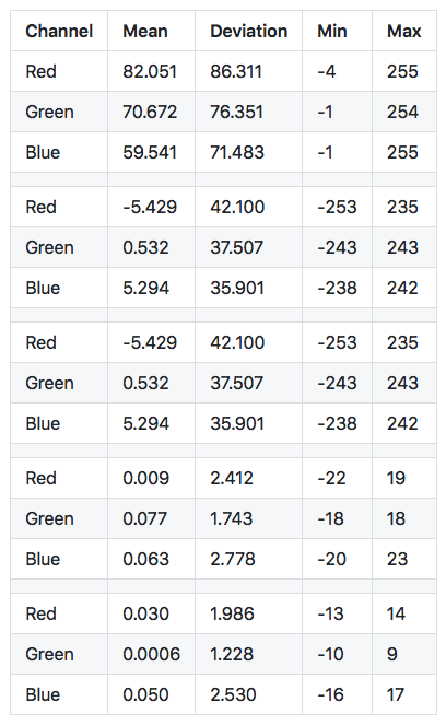
First few difference frames
Here are a few difference frames captured right after turning on the camera. Since we subtract one frame pixels from another, the value of each pixel can be from -255 to 255. The Mean will be the mean value of difference in a red, green or blue channel. Min/Max records extreme values for each frame. A few trends are immediately obvious from this data:
It takes the camera a few frames to focus on the scenery. While the camera is focusing, the difference between each frame is big, as evidenced by large values in the mean, deviation and pixel min-max range.
Once the camera is focused, the mean rapidly converges to almost zero. This will be a useful attribute for us to detect if the camera field of view has changed — we can reject all difference frames where the mean is larger than a small value like 0.1.
In a focused, stable view the min/max range becomes much smaller, just ± 20 pixels on average, and very rarely reaching ± 40 pixel intensity. That is exactly the behavior of the relatively small thermal noise present in every pixel of a camera image for which we are looking.
Zero Sequences
Let’s look at the raw data in each channel:
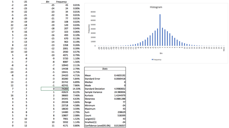
That looks like what we would expect from a random distribution of noise, yet one thing jumps out immediately — why there are so many zeroes? They are clearly breaking out from the pattern of a normal “bell curve” distribution we should expect from the physics textbook.
Looking into the raw data stream, it is quickly noticeable that each channel contains very long sequences of zeroes, sometimes going for over a hundred zeroes. Is this normal? According to our data, the probability of 0 in this sample is 14.33%. If we assume these zeroes are random, then any N-long sequence of zeroes will have a probability of 14.33% taken to the power of N.
Expected zero sequences in 518kb sample
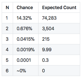
Apparently, there is virtually no chance to see a sequence of zeroes longer than 5 or 6 in our sample. Yet we are seeing sequences of 100 and more. Clearly, this is not random, and something else is going on. After digging through the data and experimenting, we found the culprit.
The problem is that a given channel has oversaturated areas. Imagine the camera focusing on an item that has bright red spots. They are so intensively red that camera will register these pixels as 255 on the red channel. Naturally, that pixel will be subject to the same noise as any other pixel, but since the signal is so strong, the next frame will still have exactly the same 255 in that pixel. In other words, for an oversaturated sensor 255 + Noise = 255, meaning that such pixels will lose the ability to register noise at all! When we subtract them from each other, we get zero, yet this zero is no longer a random thermal event - these “no-noise” zeroes simply trace the area of the oversaturated condition in the picture. That leads to a couple of important lessons:
When generating entropy with the lens uncovered, avoid too bright conditions that eliminate sensor sensitivity.
The improbably long sequence of zeroes is a telltale sign of such oversaturated spots in the difference frame. Before we generate entropy, we will scan for such improbably long sequences and eliminate them from the sample data because they contain no real thermal noise.
From our testing, we found that any matte background — like the dull finish of a MacBook Pro — works best when doing entropy generation with the lens uncovered. Or something as simple as putting your phone on the table camera up to capture a mildly lit room ceiling works well too to avoid oversaturated areas. Since we want to register as much noise entropy as we can, the ideal conditions would be to point a camera at some scenery that is “mild grey” (right in middle, around 128 on each channel), so that the camera has the full range of intensity to register noise ups and downs.
Yet before we can start generating entropy, we need to deal with one more issue.
Dealing With Correlations
Correlation is the natural enemy of entropy. When two things are correlated it means that taken together they contain less entropy then it would appear from looking at them individually. Let’s zoom in on the “pixel entropy” we generated earlier from camera noise.
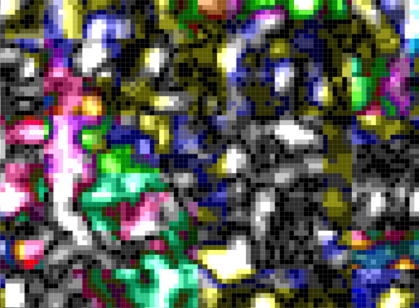
High correlation areas
As you can see, individual pixel colors do not change completely randomly. All of them are clustered in small groups few pixel wide. That makes sense: if a thermal event or high energy particle is hitting our sensor silicon somewhere, it will not hit just one and only one pixel. It will affect some area around that pixel. So all of these colors are random yet correlated. This is our first correlation factor, a correlation of space.
If we consider the implications of the original article, the second kind of correlation becomes apparent as well:
Gamma rays have far more energy than visible light photons: for example, they might have 20,000 eV compared to between 1.77 and 3.1eV for visible light from red to violet respectively. And because they have much higher energy to start with, they transfer far more to any electron they hit. This in turn then careers through the material ionising other electrons until its energy is dissipated. So an electron with 20 KeV might ionise 10,000 other electrons before it dissipates. That’s a signal that a smartphone camera ought to be able to see.
High energy particles that bombard our sensor not only affect the pixels in one frame; if the energy is high enough, it will continuously affect silicon in that area while the energy of the initial collision dissipates through the medium. Therefore some areas of our picture will have correlation going on in time through several frames.
All of these events are perfectly random, yet unless we are careful, these events will be clumped into correlated clusters. What can we do to break down such correlations as much as possible? We can reduce correlation by taking a few easy steps with our raw data:
Break local group by accessing the pixels in different order. For example, we can take all red pixels in their natural order, going from 1st pixel to the last pixel in the frame. We will take green pixels in the reverse order, going from last to 1st. For blue pixels, we can use orthogonal order that replaces rows with columns in the frame (instead of 0,1,2,3 ordering will be 0,10,20,…1,11,21…). This way correlated pixels in the clumps we have seen above will never be used together.
Instead of using frames one after another, we can use frames that are more distant from each other in time. For example, at 30 frames per second, we can buffer 15 frames, and then extract entropy by using frame 1 and 16, 2 and 17, etc. That means we will be mixing in frames that are half a second apart — which should be enough for timing correlations to dissipate away.
We will mix in red, green and blue channels in parallel from different frames, since there will be less correlation between pixels of different colors in different frames. For example the “red” pixel 10 on frame 1 is less correlated with the “blue” pixel 321 on frame 15, while it might be strongly correlated with the “blue” pixel 9, 10 and 11 in the same frame 1.
There is one caveat worth mentioning: such reshuffling and grouping of values does not eliminate correlation globally. Whatever amount of entropy we had at the beginning (reduced by correlations) in our sample, we end up with the same amount of entropy in the end, no matter how we reshuffle. What we get by accessing values across frames, in different channels, from pixels that are distant from each other is eliminating local correlation in each batch of values formed that way[2], so that each value in the batch passed to our extractor is independent from the others.
From Normal to Uniform
Now that we have all the ingredients in place, we are ready to create the entropy extractor. After correcting for oversaturated areas, the raw high-resolution data for a single channel of one frame looks like this:
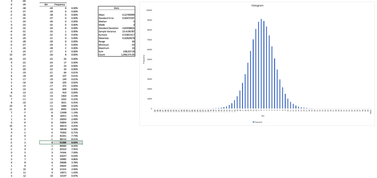
That is a perfect normal distribution of noise in our difference frame. However, to generate entropy we need to somehow convert this normal distribution to a uniform distribution. The first thought would be to use the inverse form of an elegant Box-Muller transform… which, unfortunately, wouldn’t work for us at all. The Inverse Box-Muller transform requires a continuous distribution, and our raw data is all discrete values.
In fact, the problem is even harder than it appears at first glance. Look at the numbers — despite the fact that the range of values we see in the noise is from -33 to +33, over 96% of our data points are all in the narrow range from -10 to +10. The size of that range depends on camera conditions: if a picture has too many oversaturated spots or too many dark spots [3] there will be less noise overall, and the range will decrease even further. For “lens covered” blackness the vast majority of data points can shrink to ±3: a total of just 7 different values. We need to generate perfect, uniform entropy from a limited sets of these values (around 21 values in perfect conditions, or down to 7 values in the worst conditions). And the distribution of these values will be highly biased — in our distribution, the sample zero is happening most often with a frequency of 8.69%.
How much entropy can we hope to extract, theoretically? For this purpose, there is a well-known concept of “minimal entropy” (usually referred as min-entropy). Unlike Shannon’s entropy definition, which characterizes the entropy of an overall distribution, min-entropy describes the worst case scenario — the characteristic of the value that happens most often and thus is the most predictable. In this sample, zero happens 8.69% of the time. The simple calculation of -log2(8.69%) gives us a theoretical min-entropy of 3.52 bits — the maximum number of bits we can expect to extract from a single data point. Another way of stating this: every time we read a pixel value of noise, no matter if the value is -30 or +10 or 0, reading that value reduces our uncertainty only by 3.52 bits. Despite the fact that 33 would require more than 5 bits to encode (2^5 = 32), it doesn’t matter — the only entropy (uncertainty) hidden inside each value is just 3.52 bits at best. If we have to work with worse camera conditions (i.e. less variance of noise), then our entropy per data point will go down even more. The good news is that our 12 megapixel camera has lots and lots of data points produced every second!
So, depending on camera conditions, we encode all data points into 1, 2 or 3 bits: quantized_value = raw_value % 2^bits. However, even after encoding, our bits are still heavily biased, obviously with zero bits being far more prevalent since our most common value is zero. How can we go from a zero-biased bitstream to a bitstream with uniform distribution? To solve this challenge, we are going to use the granddaddy of all randomness extractors — the famous Von Neumann extractor.
Von Neumann extractor
John Von Neumann figured out how you can get perfect entropy even if your source is a highly biased coin: a coin that lands on one side far more often then another. Let’s say we have a coin that turns up heads (0) 80% of the time, and tails (1) 20% of the time. Yet despite having a coin that is so defective, we can still extract perfectly uniform entropy from it!
Here is the key insight from Von Neumann’s extractor. Let’s think about each pair of coin tosses. Obviously, a toss of 0,0 is far more likely than a toss of 1,1 since zero is far more probable to happen. But what will be the probability of a 0,1 toss compared with a 1,0 toss? The first toss has a probability of 80% x 20% = 16%. The second toss will have probability 20% x 80% ... wait, it is the same number! We just changed the order of variables, but the result is exactly the same.
Von Neumann understood that even if your source is biased, the probability of combinations 1,0 and 0,1 are equal and you can just call the first combination the new extracted ‘zero’, and second combination an extracted ‘one’. No matter how bad your source is, the stream of ‘new’ zeroes and ones will be perfectly uniform. Here is a classical Von Neumann extractor of biased random bits:
If you have a pair of 0,0 or 1,1 just toss them away: they do not produce anything.
If you have 1,0 or 0,1 pair, use the final bit as your result and it will have a uniform random distribution: the probabilities of these two pairs are exactly the same!
The Von Neumann extractor works amazingly well and has the added benefit that we do not even need to know how biased our incoming bits are. However, we are throwing away much of our raw data (all these 0,0 and 1,1 pairs). Can we extract more entropy? Elias (’72) and Peres (’92) came up with two different methods to improve the Von Neumann extractor. We will explain Peres method since it is a bit simpler to explain and implement.
We already know that 1,0 and 0,1 have the same probability - there is no difference between 80x20 and 20x80 if a binary source is biased 80%/20%. But what about longer sequences? Let think about the “throw away” sequences 1100 and 0011. If we use straight Von Neumann method we will get nothing from these: both 11 and 00 will be tossed away. But let's calculate probabilities: 1100 will be 20x20x80x80, while 0011 will be 80x80x20x20 - the same numbers again.
There is clearly something very similar to what we have already seen. We have two sequences with the same probabilities. Again we can say that a sequence ending with 00 is a new “zero”, while sequence ending with 11 will be a new “one”. This is a case of recursion: we are using the same algorithm just on numbers doubled up instead of originals. Here is the Von Neumann extractor with simple recursion:
If you have a 1,0 or 0,1 pair, use final bit as your result (classic Von Neumann).
If you have a 1,1 or 0,0 pair, convert it into 1 or 0 and add it to a temporary buffer.
After you are done processing the initial data, run the Von Neumann extractor again on the buffer you collected.
Since all 1,1 and 0,0 sequences become just single bits, the Von Neumann classic algorithm by definition will extract more uniform bits if the initial data contained any 1,1,0,0 or 0,0,1,1. And since this algorithm is recursive we can keep running it as long as something collects in our temp buffer and extract every last bit of entropy from longer sequences. Finally, the Peres algorithm has one more abstraction that allows us to extract even more entropy from a Von Neumann source by using the position of sequences that produce bits in initial stream, which is implemented in our codebase.
Now we have a powerful extractor that can deal with an input of biased bits, and we are almost ready to extract some entropy. But there is one more step we need to do first.
Quick Test: Chi-Squared
There is no test for “true” entropy. What might look like a perfect random entropy coming from, say, quantum physics, can be in fact completely deterministically created by a software generator and fully controlled by an attacker selecting an initial seed. There is no test on the data one can run that determines a difference between a “true quantum random process” and a “software generated sequence”. The very success of modern cryptography is the fact that we can make a “software generated sequence” (the result of an encryption algorithm) look indistinguishable from “true entropy”. Yet at the same time, there are a number of software tests for randomness: FIPS-140, SP800–90B. What is going on?
To understand the purpose of such “randomness tests”, we are going to review one of the simplest tests: chi-squared (pronounced ‘kai-squared’) goodness of fit. Khan Academy has an excellent video explaining step by step how to use the chi-squared test — check it out to learn more. The chi-square test is fairly simple and consists of the following:
Formulate a theory about whatever you want to test and then calculate what you expect to observe if your idea is correct.
Observe real-world events and record the observed values.
The chi-squared statistic is calculated by summing together across all events the following: (ObservedValue - ExpectedValue)²/ExpectedValue
Use a lookup table or chi-squared calculator to answer the key question: what is the probability that the observed events are the result of your theory?
As you can see, the formula is just saying in math language “I will collect the square of all differences between what you thought was true and what is happening in the real world in the proportion of what you were expecting. If any of your expectations are too far out from reality, then the squared difference will grow very fast! The bigger it becomes, the more wrong you are.”
Let’s work it out for our case — building a uniform entropy extractor. We want to produce random bytes, that can take values from 0 to 255. We want the distribution of our bytes to be uniform, so that the probability of every byte is exactly the same. Observing every byte is an event, so we have 256 events total. Let’s say our software produced 256,000 bytes and we are ready to run the chi-square test on them. Obviously, if the bytes are uniform (our theory) we would expect to see each byte with a probability of 1/256. Therefore we will see each byte exactly 256,000/256 = 1000 times exactly. That is our expected value for each event. Then we record the observed value (how many times we actually see each byte in our data) and sum all 256 values of (ObservedValue - 1000)²/1000. That number is our chi-squared statistic. What do we do with it?
Chi-squared tables are organized by two parameters — so-called degrees of freedom — which is a fancy way of saying “a number of independent events you have minus one”. In our case, the degrees of freedom will be 256-1 = 255. The most interesting part is the second parameter P, a probability that we can calculate from 99.9% (extremely likely) to 0.1% (extremely unlikely).

The only printed table we could find tantalizingly cuts off at 250 — just 5 short from what we need! However, we can use a chi-squared calculator to get the exact values we need.
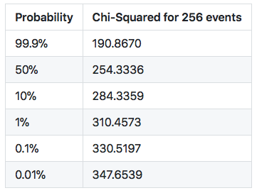
What this table tells us is the probability that our observation fits our hypothesis — the hypothesis we used to formulate all expected values. In other words, if we get chi-squared around 190, it virtually guarantees that the observed events match our theory about them — the theory that they all are coming from uniform distribution — but there’s still is a 0.1% chance that we are wrong! For a chi-squared at 284, there is a10% chance that our hypothesis is correct. That is not bad actually — if you run the chi-square test 10 times on 10 perfectly random samples, it is likely that you will get one sample around 284. If you run hundreds of random samples, one might have a chi-square value of 310, i.e. a sample with a low probability of 1%. If you willing to test a thousand samples, one might have a chi-squared value of 330 (0.1%).
As you can see, the chi-square test, like all other randomness tests, do NOT tell us anything about the nature of our randomness! They don’t tell us if it is “true” randomness or not, i.e. is it derived from a “true” physical source or generated by software. This test answers the much simpler question: after looking at the given sample, what is the chance that this sample of random values came from a source with uniform distribution?
Since the tests are probabilistic in nature, care must be taken in interpreting the results. It doesn’t mean that something is obviously “wrong” with a chi-square score of, say 310 (which is a low 1% probability). It takes just a few tries of running this script to produce chi-square scores over 300 (as measured by ent) from the state of the art /dev/urandom on Mac OS X. If you keep repeating the test dozens or even hundreds of times, you should expect less and less likely values to manifest.
for i in {1..10}; do dd if=/dev/urandom bs=1k count=1k &> /dev/null | ent -t | cut -d, -f4; done
194.700684 308.307617 260.475586 236.611328 316.724609 306.418945 262.301270 240.013184 205.627930 257.049805
However, the probability is going down fast above 330. The probability of chi-squared 400 is just 0.000001% — it might happen just once per 100 million of samples!
The chi-squared test will be our early warning radar when something breaks down in our extractor. The test tells us “hey, this looks less and less likely that your bits are coming from a uniform source!” if the chi-square score is rising. It states nothing about the nature, validity or source of our entropy, only how likely it is that the bits are produced by a uniform random source.
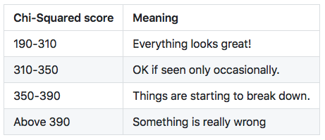
We will use the chi-squared statistic of entropy block as a real-time quality score, and we will run a more compressive randomness test suite later when we evaluate the final results.
All Together At Once
As we have seen, a good entropy extractor is quite a complicated piece of crypto machinery! Let’s review how we put all the pieces together:
Take two video frames as big arrays of RGB values.
Subtract one frame from another, that leaves us with samples of raw thermal noise values.
Calculate the mean of a noise frame. If it is outside of ±0.1 range, we assume the camera has moved between frames, and reject this noise frame.
Delete improbably long sequences of zeroes produced by oversaturated areas. For our 1920x1080=2Mb samples and a natural zero probability of 8.69%, any sequence longer than 7 zeros will be removed from the raw data.
Quantize raw values from ±40 range into 1,2 or 3 bits: raw_value % 2^bits.
Group quantized values into batches sampled from different R,G,B channels, at big pixel distances from each other and in different frames to minimize the impact of space and time correlations in that batch.
Process a batch of 6–8 values with the Von Neumann algorithm to generate a few uniform bits of output.
Collect the uniform bits into a new entropy block.
Check the new block with a chi-square test. Reject blocks that score too high and therefore are too improbable to come from a uniform entropy source.
Whew! That was simple.
Generating Entropy
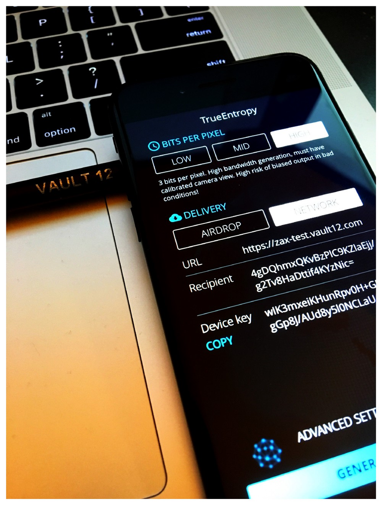
All right, let’s generate some hardcore “true” entropy! The iOS app is here or you can compile it from the source code and trace every bit as it travels through the extractor. There are two ways to get entropy from the app: AirDrop it to your MacBook (and we included the option to upload entropy block as CSV file as well for manual analysis), or use a Zax relay for secure device-to-device upload, which we will cover later.
If the camera view is good, simply run the extractor at the maximum bandwidth by extracting all 3 bits from each noise value.
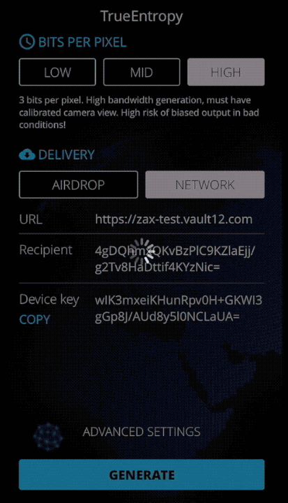
However, things break down fast if the picture quality goes bad, by over saturation or having too many dark areas where noise variance goes down. With less variance, taking 3 bits from each datapoint will feed a lot of garbage into the extractor. The Von Neumann algorithm is not magic, and it will not create entropy out of thin air if we are oversampling raw data points[4]. Chi-squared statistics capture that immediately.
3 Bit Oversaturated
The fix is easy — if picture quality is poor, just reduce the number of bits extracted from each datapoint down to 2 bits or even 1 bit. For this view, reducing it down to 2 bits returns our extractor back to normal scores.
2 Bit Oversaturated
In truth, it is far simpler to run this extractor with excellent quality and maximum bit extraction, but it doesn’t make for an exciting video. Here is one of the best conditions we found to set up the camera for a perfect noise capture.
3 Bit MacBook Grey
All this required was the high tech equipment of a pencil that lifts up the camera just a bit above a MacBook’s dull grey surface. It is the perfect scenery to capture our full range of thermal noise[5].
High tech entropy generation with a pencil
Sending Entropy
Of course, all this firehose of perfect thermal entropy would be of little use if it stays local to your device. The good news is, we have already built the Zax relay around the top tier NaCl library to serve asynchronous, anonymous and encrypted process-to-process communications. That allows us to encrypt thermal entropy (produced by the owner in a condition they fully control) and establish a secure channel through a NaCl relay to send this entropy to any device that the owner selects. This will get us NaCl 256-bit “computational security” for such networked entropy sources. Each device is addressed by a NaCl public key. Relays do not use public keys of the communicating devices directly, the relay address space is defined as a “hash of the public key” (hpk). The communications are encrypted twice — the inner layer is encrypted with whatever is the destination public key by the originating device (i.e. our relays never even see the raw data), and the outer layer is encrypted with a separate NaCl ephemeral session key created when a station connects to relay. If you want to learn more about Zax relays, you can read about our full crypto architecture as well as our new protocol for large file exchange.
Using a Zax relay you can run a process inside a cloud server that directly receives encrypted entropy from an Apple device under your control, unpack it in memory, and use that entropy as the situation demands — to seed local /dev/urandom as an extra source or to establish a separate, owner-controlled entropy pipeline directly from camera thermal noise.
But isn’t this a bit of circular logic — using servers to secure servers? If you think through practical implications, it’s actually not. The main reason we put servers in the cloud is to process heavy computational load and to have access to a high bandwidth connection. The individual relay that passes entropy to cloud servers does not need heavy computing power nor high bandwidth, so it doesn’t need to be hosted in the cloud! As matter of fact a relay can be run on a modest Raspberry Pi stuffed into the same closet as an iPhone generator. With both the relay and iPhone under full owner control, the owner can establish a strong, secure channel into the cloud server environment. The only assumption we need to make is that owner’s SSH keys and server entropy during initial setup (server-side SSH keys) were not compromised, and that the owner can securely transfer a private key to the cloud server to establish a secure channel with the relay.
Here is how it all fits together:
To work with a Zax relay you need to install the Glow client library: npm i -g theglow.
Pick a secret key for your target device or server. This can be any random 32 bytes generated anyway you like. For example, generate a key file cat /dev/urandom | head -c 32 | base64 > station_key.txt on a secure machine and use that file on a single target server. You can also use TrueEntropy’s “AirDrop” mode to generate the initial key entropy directly.
Init a station with that key: cat station_key.txt | glow key --set. Or you can use glow key --generate to avoid creating an extra file. That command will also print out the resulting public key.
Copy your device public key (PK): glow key --public
Paste that public key in the Recipient slot of the TrueEntropy app and specify a relay URL.
Copy the Device Key from the TrueEntropy app.
Download the encrypted blocks uploaded by the TrueEntropy app, for example to download 5 blocks at once: glow download https://zax-test.vault12.com [Device/Sender Public Key] -n 5 We used our test relay in this example[6], for any production use you should deploy your own relays from source. For direct entropy use, you can pipe it into any destination: glow download https://zax-test.vault12.com [Device/Sender Key] --silent --stdout | ent
That’s it! As long as TrueEntropy is running in “Network” mode, it will be uploading encrypted blocks to your relay, which in turn you can download, decrypt on a target device, and use as you see fit.
If you are planning to use this for any practical purpose other than research, make sure you take care in selecting a good view for your camera (or reduce TrueEntropy’s bit setting to 1-2 bits), enable chi-square cutoff in Advanced settings, and use some form of hashing on the destination machine before using each entropy block. Keep in mind TrueEntropy is a research prototype, and we do not recommend using it in actual production environment.
The Real Test: SP800–90B
Now we know how to generate and deliver entropy to any device. But besides a simplistic test of chi-squared goodness of fit, how do we know whether the entropy we have produced is any good? Thankfully the good folks at NIST have already been thinking for a long time about how to build and evaluate entropy extractors, and they have summarized all the best practices in the SP800–90B document[7]. This is a must-read resource for anybody who is interested in serious work around writing randomness generators and entropy extractors.
Many of the SP800–90B tests are implemented in software, and anybody can run them on any entropy source. These tests do a lot of heavy lifting checking for patterns far above and beyond our simple chi-squared test — it takes many hours for this test suite over single file. So how does a TrueEntropy block stack up against a state of the art entropy test suite?
python iid_main.py ~/entropy-3b1.bin 8 -v
reading 2097152 bytes of data
Read in file /home/fallout/entropy-3b1.bin, 2097152 bytes long.
Dataset: 2097152 8-bit symbols, 256 symbols in alphabet.
Output symbol values: min = 0, max = 255
Calculating statistics on original sequence
Calculating statistics on permuted sequences
permutation tests: 99.99 percent complete
statistic C[i][0] C[i][1]
excursion 3845 0
numDirectionalRuns 8304 3
lenDirectionalRuns 82 854
numIncreasesDecreases 5930 10
numRunsMedian 8144 2
lenRunsMedian 2288 1720
avgCollision 9654 0
maxCollision 433 204
periodicity(1) 1455 29
periodicity(2) 28 1
periodicity(8) 2996 32
periodicity(16) 8229 35
periodicity(32) 41 3
covariance(1) 229 0
covariance(2) 799 0
covariance(8) 421 0
covariance(16) 7136 0
covariance(32) 3487 0
compression 7488 6
(* denotes failed test)
** Passed IID permutation tests
Chi square independence
score = 65162.2, degrees of freedom = 65535, cut-off = 66659.4
** Passed chi-square independence test
Chi square goodness-of-fit
score = 2285.22, degrees of freedom = 2295 cut-off = 2510.06
** Passed chi-square goodness-of-fit test
** Passed chi square tests
LRS test
W: 5, Pr(E>=1): 0.864829
** Passed LRS test
IID = True
min-entropy = 7.92358
Perhaps these tests are so easy to pass that anything will cross that threshold? As it turns out, that is not the case. For a quick experiment we replaced out the Von Neumann extractor with a far simpler one: it looks at noise value and outputs 1 if it is above zero, and 0 if it is below zero. Since (unlike Von Neumann) we never skip any sequences other than zero values, this extractor produces twice as much output (we included it in the source code as a reference). The bell curve distribution we have shown above is almost perfectly symmetrical, so it should be pretty random if the value is above or below zero, right? Would it be a good extractor and have higher performance?
The SP800–90B judgement is harsh: such a naive extractor immediately fails no fewer than 5 tests:
$ python iid_main.py ~/entropy-direct.bin 8 -v
reading 1999996 bytes of data
Read in file /home/fallout/entropy-direct.bin, 1999996 bytes long.
Dataset: 1999996 8-bit symbols, 256 symbols > in alphabet.
Output symbol values: min = 0, max = 255
Calculating statistics on original sequence
Calculating statistics on permuted sequences
permutation tests: 99.99 percent complete
statistic C[i][0] C[i][1]
excursion 7875 0
numDirectionalRuns* 10000 0
lenDirectionalRuns 6435 3562
numIncreasesDecreases 394 4
numRunsMedian* 10000 0
lenRunsMedian 40 48
avgCollision* 10000 0
maxCollision 5222 1236
periodicity(1)* 0 0
periodicity(2) 46 2
periodicity(8) 1955 39
periodicity(16) 512 15
periodicity(32) 7632 39
covariance(1)* 0 0
covariance(2) 141 0
covariance(8) 6251 0
covariance(16) 5847 0
covariance(32) 5980 0
compression 7540 3
(* denotes failed test)
** Failed IID permutation tests
IID = False
Can we reliably use a 3-bit Von Neumann extractor with a good camera view? We definitely can, here is another entropy block produced with 3-bit settings on a balanced camera view:
python iid_main.py ~/entropy-3b2.bin 8 -v
reading 2097152 bytes of data
Read in file /home/fallout/entropy-3b2.bin, 2097152 bytes long.
Dataset: 2097152 8-bit symbols, 256 symbols in alphabet.
Output symbol values: min = 0, max = 255
Calculating statistics on original sequence
Calculating statistics on permuted sequences
permutation tests: 99.99 percent complete
statistic C[i][0] C[i][1]
excursion 5990 0
numDirectionalRuns 6878 8
lenDirectionalRuns 939 5563
numIncreasesDecreases 1204 13
numRunsMedian 220 1
lenRunsMedian 1198 966
avgCollision 8953 0
maxCollision 6838 1137
periodicity(1) 909 16
periodicity(2) 3748 45
periodicity(8) 8752 22
periodicity(16) 9318 16
periodicity(32) 8374 20
covariance(1) 3183 0
covariance(2) 4537 0
covariance(8) 3617 0
covariance(16) 2460 0
covariance(32) 316 0
compression 1473 6
(* denotes failed test)
** Passed IID permutation tests
Chi square independence
score = 65285.8, degrees of freedom = 65535, cut-off = 66659.4
** Passed chi-square independence test
Chi square goodness-of-fit
score = 2269.05, degrees of freedom = 2295 cut-off = 2510.06
** Passed chi-square goodness-of-fit test
** Passed chi square tests
LRS test
W: 4, Pr(E>=1): 1.000000
** Passed LRS test
IID = True
min-entropy = 7.90724
Good news — our extractor output passed the SP800–90B IID test.[7]
Future Improvements
What started as a fun weekend project turned out to be an interesting application, and we ended up spending over a week to implement it to the level of a minimal MVP. It once again showcased the amazing power contained in billions of smartphones that we take for granted these days. Of course, the first MVP might be too raw for production use. The good news is, all our source code is MIT licensed, so you are welcome to take a stab at making it better. Someday, you can replace your expensive wall of lava lamps with a simple used iPhone in the closet!
What can be done to improve this codebase:
We are taking the camera as a given constant, yet it is quite configurable and an extremely powerful device! What camera settings can be adjusted and automated to maximum noise variance in all conditions? The app will then be less sensitive to selecting a proper view and can just adjust itself to generate perfect entropy in any conditions.
We used the Von Neumann extractor since it was the simplest to implement and it offered a perfect educational canvas to demonstrate how each bit sequence is converted from biased raw source to uniform. However, cutting-edge extractors in the industry leverage “sum-product theorem” (sources are mixed up as X*Y+Z over specific field) and might be much more powerful given the number of noise pixel values we are getting from each frame.
Want to relax IID assumptions and avoid careful setup of a non-correlated quantizer? Easy — use any good universal hash function. The only new requirement is that the universal hash will require a one-time seed. We can make an easy assumption that the iPhone local state of /dev/urandom is totally independent from thermal noise camera is seeing, and simply pick that seed from everybody's favorite CSPRNG.
We are not actually extracting the maximum amount of entropy. Newer iOS devices support HD resolution of 3840x2160 per frame. The higher the resolution, the more variance of each pixel noise the camera will detect, and we can even start extracting 4-bit datapoints in the same “perfect” conditions. The downside is that now the device has to process 8Mb of data before the the first bit of entropy is generated, and it slows down initial output and requires a huge memory footprint. We left the default at 2Mb per frame for better responsiveness, but you are welcome to change that if you are looking for maximum entropy throughput[8].
Not surprisingly, most of the cycles in our app are spent on running the extractor logic on the iOS device CPU — that is by far the main performance bottleneck in the app right now. Calculating the frame difference noise takes only 0.1 seconds on the iPhone7 over a 2Mb frame, while running the extractor over the same frame takes up to 5–7 seconds. To maximize the bandwidth of thermal entropy, one solution would be only capture raw noise values from the iPhone and run the extractor on the target machine. Such a setup would allow us to generate entropy at a theoretical maximum speed for camera resolution in the tens of megabytes per second.
The chi-square test is the simplest and quickest realtime tests we can run as entropy blocks are generated. The SP800–90B we used for static testing has a massive array of entropy assessment and health algorithms. Adding a few realtime health checks, the SP800–90B suite can provide additional safeguards when used in production.
One More Thing
Well, that is it! We hope you enjoyed our quick foray into randomness extraction that holds interesting possibilities to generate a massive amount of entropy from any smartphone with a camera.
One of our goals in creating the TrueEntropy app was to stress test our relay network to see how it behaves under the heavy load from handling all these endless entropy streams. These relays power our main project which we have run in stealth mode for a while, but we are just about to open it up for a public beta test.
One of the big problems facing all owners of cryptocurrencies is that there is no good way to securely and reliably store extremely valuable private keys and seed phrases. For many years, state of the art security was to print out a 12-word phrase and keep it in a bank safety deposit box[9]. We started Vault12 to build a much better platform to secure crypto-assets, and in our next essay we will tell you all about it! If you are interested in cryptography and cryptocurrencies, we would love to have more beta testers for the upcoming public beta of our platform — feel free to join our Slack if you want to participate!
-Team Vault12
Many thanks to Terence Spies, Yevgeniy Dodis, Lucas Ryan and Naval Ravikant for reading the draft of this essay and valuable feedback.
References
An introduction to randomness extractors https://cs.haifa.ac.il/~ronen/online_papers/ICALPinvited.pdf
Von Neumann Extractor: https://cs.nyu.edu/courses/spring06/G22.3220-001/scribe/Lecture2.pdf http://www.eecs.harvard.edu/~michaelm/coinflipext.pdf
Elias & Peres Extractor: https://ocw.mit.edu/courses/electrical-engineering-and-computer-science/6-441-information-theory-spring-2016/lecture-notes/MIT6_441S16_chapter_28.pdf
Extracting Randomness Using Few Independent Sources http://www.boazbarak.org/Papers/msamples.pdf
Zax “NaCl” Relay
https://github.com/vault12/zax
Zax Technical Spec
https://s3-us-west-1.amazonaws.com/vault12/crypto_relay.pdf
Glow Client Library
https://github.com/vault12/glow
Your Smartphone Can Measure Your Radiation Exposure https://medium.com/the-physics-arxiv-blog/your-smartphone-can-measure-your-radiation-exposure-ce9b464d68aa
One of the Secrets Guarding the Secure Internet Is a Wall of Lava Lamps
https://sploid.gizmodo.com/one-of-the-secrets-guarding-the-secure-internet-is-a-wa-1820188866
Entropy Attacks!
https://blog.cr.yp.to/20140205-entropy.html
SP800–90B
https://csrc.nist.gov/CSRC/media/Publications/sp/800-90b/draft/documents/sp800-90b_second_draft.pdf
Managing and Understanding Entropy Usage https://www.blackhat.com/docs/us-15/materials/us-15-Potter-Understanding-And-Managing-Entropy-Usage.pdf
Avalanche Effect Generators
http://holdenc.altervista.org/avalanche/
http://ubld.it/truerng_v3
Red Hat: Passing entropy to guest OS
Amazon HSM
[1] Copy two blank pictures from the camera as layers, set layer blending to “Difference” and adjust “Levels” to about 20x amplification.
[2] Each value in a batch becomes locally IID (independent identically distributed). There are computationally slower methods to build quantizer that satisfies a ‘global’ IID condition, but practically it is much simpler to deal with residual correlations by simply passing extractor output through a hash function.
[3] The variance of sensor noise is correlated with the amount of light hitting the sensor — a higher intensity produces more noise as long as area is not oversaturated, while dark spots produce smaller variance of noise values
[4] Formally speaking, by oversampling values that do not have enough variance we are breaking the IDD assumption about our data points that requires the Von Neumann/Peres algorithm to work — a number of bits in oversampled values becomes predictable.
[5] Another option we found is to put the phone on the desk camera up to focus on a ceiling in a dimly lit room.
[6] We restart and update that zax-test server quite often. You are welcome to use it for quick testing but don’t expect any sort of stable performance from that URL! It can and will go offline/restart at any moment.
[7] Since our essay is getting quite long, for brevity we are showing only quick tests of the VN/Peres extractor. For additional scrutiny you can export raw values from the Sample class and run non-IID tests to measure characteristics of raw thermal data (and its entropy) — SP800–90B has a lot of details on how to conduct comprehensive testing of raw non-IID data.
[8] Change line 16 in Constants.swift to AVCaptureSession.Preset.hd4K3840x2160
[9] As some Ƀ owners painfully found out during the Greece banking crisis, when banks close, they close access to safe deposit boxes — exactly when owners needed them the most.![]
FIRST PUBLISHED https://medium.com/vault12/how-to-get-true-randomness-from-your-apple-device-with-particle-physics-and-thermal-entropy-a9d47ca80c9b
Hi! I am a robot. I just upvoted you! I found similar content that readers might be interested in:
https://medium.com/vault12/how-to-get-true-randomness-from-your-apple-device-with-particle-physics-and-thermal-entropy-a9d47ca80c9b