Hi Everyone,
Welcome to the seventh post in my conference and journal paper post series. This series will contain ten conference and journal papers from my time working in the Queensland Government. In my post, My Peer Reviewed Conference and Journal Papers, I explain the purpose of this series.
Calculation of Transport Mode Shift in the Absence of Complex Transport Models was the other paper that I presented at the 2014 ARRB Conference. This was my most technical conference paper. It was heavily geared towards economists with considerable experience in project evaluation and cost benefit analysis as well as transport modellers.
Transport projects can be highly complex, and their impacts are not always easy to predict. Hence, we have transport modellers who use sophisticated transport modelling software. Such transport modellers are expensive to hire, and the process of transport modelling is time consuming. The outputs of transport modelling are also geared towards engineering rather than economic analysis. Therefore, transport modelling may need to be run again to obtain outputs required by economists to conduct an economic evaluation or cost benefit analysis. This might be visible for very large projects that require a detailed economic analysis; this might also include a general equilibrium analysis to determine the broader impacts on the economy. For even multi-million dollar transport projects, this would not be done. Therefore, a cost benefit analysis would have to rely on very loose assumptions.
To improve the quality of these assumptions, I developed a simple methodology using triangle distributions. Triangle distributions enable simple modelling using Microsoft Excel spreadsheets with only a moderate compromise to the accuracy of the modelling when compared to sophisticated software that uses normal or complex skewed distributions.
I had no problems receiving approval from Transport and Main Roads, and the paper was well received by the ARRB Conference. Unfortunately, this methodology was not adopted for the purpose of rapid modelling for cost benefit analysis, but similar models may be in use for the purpose of helping engineers refine the project design. This paper could have provided some input for them.
CALCULATION OF TRANSPORT MODE SHIFT IN THE ABSENCE OF COMPLEX TRANSPORT MODELS
ABSTRACT
The extent of mode shift induced by any transport initiative is often an essential input to an economic appraisal. Transport modelling is often time consuming and expensive. Transport modelling is often not available at the earlier planning stages and sometimes not available at all for some projects. To address the often lack of availability of data from sophisticated transport models, a simple methodology to determine mode shift has been developed. This paper explains the methodology to determine mode shift and the applications for this methodology to CBA models.
The methodology applies triangle distributions of perceived costs for travel for various modes. The interaction of these triangles determines the number of commuters utilizing each mode from the calculated integrals of the triangle distributions (two linear functions). The triangles were constructed using maximum, minimum and mean values for perceived costs. Triangle distributions were selected mostly due to the ease of manipulation using maximum, minimum and mean values.
The triangle distribution methodology has been applied to a non-infrastructure model (TRIMM). This model was designed to evaluate non-infrastructure solutions for road and transport. Detailed modelling is rarely available for non-infrastructure solutions. The application of the triangle distribution methodology was deemed an appropriate solution for the TRIMM model considering the success of many non-infrastructure solutions for transport relies upon mode shifts. The application of the triangle distribution methodology can potentially extend beyond just transport and road projects to any analysis of behaviour that can be defined within a set of parameters.
1. INTRODUCTION
The extent of mode shift induced by any transport initiative is often an essential input to an economic appraisal. Transport modelling is often time consuming and expensive. Transport modelling is often not available at the earlier planning stages and sometimes not available at all for some projects. To address the often lack of availability of data from sophisticated transport models, a simple methodology to determine mode shift, referred to as the Tri Methodology in this paper, has been developed. This paper explains how the Tri Methodology was developed to determine mode shift and the applications for this methodology to cost benefit analysis (CBA) models.
The development of the Tri methodology involved a number of key steps. These include determining the most appropriate distributions of costs, the interaction between distributions of cost of different modes, selecting appropriate unit values for costs and determining a range for these costs. A number of distributions were considered and assessed according to likely best fit, ease of manipulation into a model and ease of application to current data and information. The interaction between the distributions for different modes of transport has been used to determine mode shift when an element relating to perceived costs changes. For example, an increase in bus fare will shift the bus distribution of perceived costs to the right1 increasing the percentage of commuters that would prefer to travel by car. Unit values have been adopted from Part 4 of The Australian Transport Council (ATC) Guide to Project Appraisal (2006) and Part 4 of Austroads Guide to Project Evaluation (2012). These values have been used to determine the mean, minimum and some of the maximum values for the perceived cost distributions for each mode.
2. PERCEIVED COST FUNCTIONS
Perceived costs are the costs users consider when making travel choices; these typically include fuel cost, tolls, and parking (TRT Trasporti e Trerritorio SRL 2012). Road user behaviour is determined by the road user’s perceived costs of travel. Perceived costs vary depending on the mode of transport. The perceived costs for travelling by bus are typically the bus fare and the value of time. Perceived value of time varies depending on how this time is spent. Value of time spent waiting, could be different to that spent on the bus or walking to the bus stop. Part 4 of the ATC guidelines states a formula for the perceived cost of travelling on public transport; this formula is stated in Equation 12 .
Equation 1
PC=F+V×[(TA×WA)+(TW×WW)+(TR×WR)+(TI×WI)+N×(TP+(TAT×WAT)+(TWT×WWT))]
Where:
PC = total perceived cost (generalised cost)
F = Fare ($)
V = standard value of time ($/min of, say, in-bus time or some other benchmark)
TA = access time i.e. between an origin/final destination and the public transport facility (mins)
WA = weighting on access time (to reflect its perceived valuation relative to in-bus travel time)
TW = (expected) waiting time at a bus stop or train station for initial boarding (mins)
WW = weighting on expected waiting time (to reflect its perceived valuation relative to in-bus travel time)
TR = unexpected waiting or travel (associated with service unreliability)
WR = weighting on unexpected waiting or travel time
TI = in-vehicle time (mins)
WI = weighting on in-vehicle time to reflect quality attributes (relative to in-bus travel time)
NT = number of transfer
TP = weighting on in-vehicle time to reflect the inconvenience associated with a transfer (in equivalent in-bus travel time (minutes)) where an interchange occurs
TAT = access/walk time on transfer
WAT = weighting on transfer access/walk time
TWT = waiting time on transfer
WWT = Weighting on transfer waiting time
Source: Australian Transport Council (2006), National Guidelines for Transport System Management in Australia: Part 4 Urban Transport, Page 20
A similar formula for perceived costs can be constructed for private car use; the formula applied to the Tri Methodology is stated in Equation 2.
Equation 2
PC=T+P+V×((TI×WI)+(TR×WR))+(FCR×FCP)+(TWR×TWP)
Where:
PC = total perceived cost (generalised cost)
T = Toll ($)
P = Parking ($)
TI = in-vehicle time (mins)
WI = weighting on in-vehicle time to reflect quality attributes (relative to in-car travel time)
TR = unexpected waiting or travel (associated with service unreliability)
WR = weighting on unexpected waiting or travel time
FCA = fuel costs per trip (resource cost)
FCP = percentage of fuel costs perceived (greater than 100%, includes fuel tax)
TWA = tyre wear costs per trip (resource cost)
TWP = percentage of tyre wear costs perceived (less than 100%, costs not directly associated with trip)
3. COMPARISION AND SELECTION OF DISTRIBUTIONS
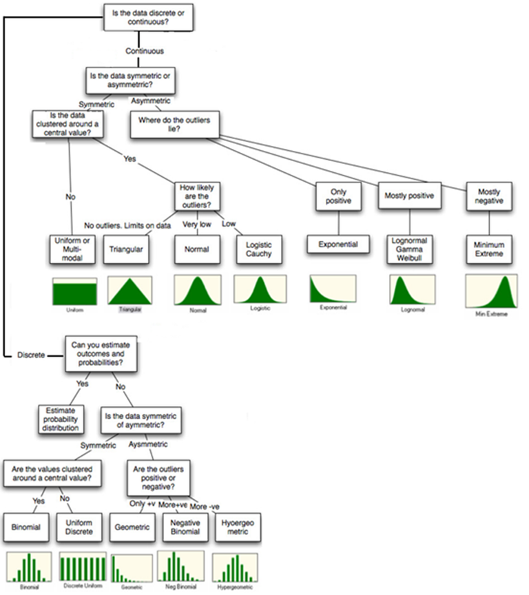
There are numerous types of distributions that can be applied to sets of data. Distributions of data can be categorised as discrete or continuous, symmetric or asymmetric, clustered around a central value or widely dispersed, and has limits or includes outliers. Perceived cost distributions can be considered as continuous distributions defined within limits. As perceived costs relate to human behaviour, they are likely to have a central tendency following a distribution close to that of a normal distribution (Hausman and Wise 1976 and Department for Transport 2014a). The maximum and minimum perceived costs per component valued in Part 4 of the ATC Guide to Project Appraisal indicate perceived costs are close to a symmetrical distribution. Damodaran (2007) summarized the appropriate application of distributional choice; this summary is presented in Figure 1.
If one considers perceived cost distributions to have symmetrical central tendencies with few outliers, applying Damodaran’s logic, perceived costs for travel are most likely to be appropriately represented by a normal or triangle distribution. For a normal distribution, the mean and variance need to be estimated. For a triangle distribution, the mean, minimum and maximum values need to be estimated. The ATC values could be adopted as the mean values and the ‘out of pocket’ outgoings of a commute such as fares, tolls and parking fees can be used to determine the minimum values. Additional research is required to determine variance and maximum values. In regards to mathematical complexity, triangle distributions are easier to manipulate to derive results. Triangle distributions can also be easily skewed, if needed, using higher maximum values. A disadvantage of using a triangle distribution compared to using a normal distribution is that outliers will not be recognized, this problem is addressed in Section 7 of the paper. The triangle distribution is sometimes referred to as the ‘lack of knowledge distribution’, which seems appropriate considering the methodology is only intended to provide a rough gauge of mode shift.
Data limitations present problems determining the distribution of preferences. For transport initiatives, data is normally available regarding the number of commuters using particular modes of transport but data is not available regarding the sensitivity of commuters to particular upgrades. There are numerous published reports and papers outlining perceived costs for various modes of transport.
Figure 1: Selection of Appropriate Distribution
Source: Damodaran, A. (2007), Statistical Distributions, Figure 6A.15 Distribution Choices
Minimum, maximum and mean figures are available for some perceived cost components as well as the perceived cost functions. Distributions of perceived costs could be built around these values. The maximum, minimum and mean perceived costs can be calculated using base case data that includes distance travelled, operating speed, tolls, fares, etc…. The triangle perceived cost distribution could be used to derive the number of base case commuters per mode. The number of commuters derived can be compared to the actual number of commuters. If the numbers are close, project case data can be entered using the same maximum, minimum and mean values as the base case. If the numbers are different, the perceived costs will need to be calculated using different maximum, minimum and mean values.
For the Tri Methodology, to address the problem of derived results not matching base case data, the maximum values for each mode can be adjusted by a percentage; the minimum and mean values are held constant. The maximum values are more likely to have a larger range than the minimum values or mean values as the maximum perceived costs are not restricted by an upper bound. The minimum values have been held constant as the variation in minimum value is expected to be small. The minimum value will not fall below the assumed ‘out of pocket’ perceived costs such as tolls, parking and fares, or be greater than the mean value. The ATC guideline values have been adopted as the mean values applied to this methodology; these values are consistently applied across many Australian road and transport agencies. Two adjustments to the maximum value equates to 9 iterations for 2 mode types and 27 iterations for three mode types3 . Increasing the number of iterations of calculations adds complexity and size to the model with diminishing returns to accuracy.
4. METHODOLOGY OF DISTRIBUTING PERCEIVED COSTS
Given that some commuters use public transport while others use private cars, one can assume that not all commuters have the same perceived costs. For simplicity, perceived costs have been segregated based on extent of subjectivity. The ‘out of pocket’ perceived costs such as fares, tolls and parking fees have been treated as the minimum perceived costs for a trip. Values defined as mean and maximum values in the ATC guidelines or Austroads reports have been used to determine the mean and maximum perceived cost values respectively.
For commuters taking public transport, fares4 are assumed to have the same perceived value per zone for all commuters but all other perceived costs are subject to the commuter’s value of time. Therefore, we can assume the minimum perceived cost of public transport is equal to the fare. Part 4 of the ATC guidelines has a range of values for weighting various travel time components. These components have been used to determine the maximum and mean perceived costs for travelling by bus.
For commuters travelling by private car, tolls and parking fees5 are generally less subjective for commuters, whereas travel time and perception of vehicle operating costs (VOC) are more subjective and may have a large degree of variance. Therefore, we can assume the minimum perceived cost of private car travel is equal to tolls and parking fees. To be included in addition to the price of tolls and parking, a mean perceived cost of travel by private car can be derived by including the Austroads values for travel time costs, fuel costs and tyre wear costs. In additional to the resource costs quoted by Austroads for fuel costs, fuel taxes needs to be incorporated. The tyre wear costs will need to be adjusted downwards as infrequent purchase of tyres diminishes the extent tyre wear costs are perceived. The maximum perceived costs for travelling by private car cannot be derived from the currently available parameters. Therefore, the maximum value for private cars has been calculated by applying the same percentage increase in mean value applied to the public transport maximum perceived cost value. To improve the accuracy of the maximum value, current commuter behaviour should be considered.
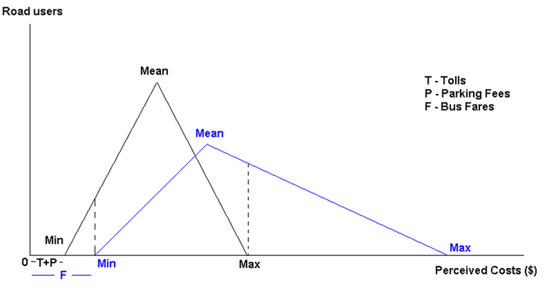
Using the preferred triangle distribution described in Section 3, perceived cost equations in Section 2, and the mean, maximum and minimum values described in this section; the distributions of perceived costs should resemble those shown in Figure 2.
Figure 2: Triangle Distribution of Perceived Costs of Buses and Private Cars
Legend:
- Black triangle distribution represents the perceived costs of travelling in private cars
- Blue triangle distribution represents the perceived costs of travelling in buses
- The dotted line is used to match the minimum or maximum perceived costs of one mode with the coinciding perceived costs of another mode
The distributions of perceived costs shown in Figure 2 can be derived using the minimum, mean and maximum perceived costs. Each triangle consists of two functions, one function from minimum to mean and another from mean to maximum. Each function can be written in the form Y=α+βX, where Y= commuters, X=Perceived Costs, α=Y-Axis Intercept and β is the sensitivity of vehicle usage to perceived costs (gradient); Y and X are variables while α and β are parameters. For the function between minimum perceived costs and mean perceived costs, β is derived according to the formula in Equation 3 and α is derived according to the formula in Equation 4.
Equation 3
β1=(RUT×2/(PCmax-PCmin))/(PCmean-PCmin)
Equation 4
α1=-β1×PCmin
Where:
RUT = total number of commuters
PCmax/min/mean = maximum, minimum and mean perceived costs for using transport
For the function between mean perceived costs and maximum perceived costs, β is derived according to the formula in Equation 5 and α is derived according to the formula in Equation 6.
Equation 5
β2=-(RUT×2/(PCmax-PCmin))/(PCmax-PCmean)
Equation 6
α2=-β2×PCmean+(α1+β1×PCmean)
The interaction between the triangles can be used to estimate the number of commuters expected to travel by car or bus along a particular route. A simple approach to determine these numbers would be to consider the probability that the perceived cost of travel for one mode of transport is less than the other mode. In reference to Figure 2, the area beneath the private cars perceived cost distribution between the minimum perceived costs for private cars and buses represents commuters that will prefer to travel by private car regardless of their perceived cost of travelling by bus, see Equation 7. The areas beneath the perceived cost distributions between the minimum perceived cost for buses and the maximum perceived cost for private cars can be used to determine the expected number of commuters that travel by private car or bus when the probability for commuters travelling by bus is greater than zero, see Equations 8 and 9. The percentage overlap of the distributions of commuters travelling by each mode is used to calculate the number of commuters travelling by each mode, see Equation 10.
Equation 7
RUPB=0 = MinB∫MinP(α1P+β1PXP)dx
Equation 8
RUPB>0 = Min(MeanP, MaxB)∫MinB(α1P+β1PXP)dx + Max(MeanP, Min(MaxP, MaxB))∫MeanP(α2P+β2PXP)dx
Equation 9
RUBB>0 = MeanB∫MinB(α1P+β1PXP)dx + Min(MaxP, MaxB)∫MeanB(α2P+β2PXP)dx
Equation 107
RUP = RUPB=0 + (RUT – RUPB=0) × RUPB>0/(RUPB>0 + RUBB>0)
Where:
RUP = commuters travelling by private car
RUPB>0 = maximum number of commuters that could travel by private car when probability of travelling by bus is greater than zero
RUBB>0 = maximum number of commuters that could travel by bus when probability of travelling by bus is greater than zero and the probability of travelling by private car is less than one
RUPB=0 = commuters travelling by private car when probability of travelling by bus is zero
RUT = Total number of commuters
XP/B = perceived costs of using private cars or buses
MeanP = mean perceived costs of using private cars
MinP = minimum perceived costs of using private cars
MaxP = maximum perceived costs of using private cars
MeanB = mean perceived costs of using buses
MinB = minimum perceived costs of using buses
MaxB = maximum perceived costs of using buses
The commuters travelling by bus (RUB) can be calculated by subtracting commuters travelling by private car (RUP) from the total number of commuters (RUT). Equations 7 to 10 hold true if the minimum perceived cost for travelling by private car is less than the minimum perceived cost for travelling by bus. If the perceived cost for travelling by bus is less than that of travelling by private car, Equations 7 to 10 can be applied to calculate the number of commuters expected to travel by bus by substituting the parameters for private cars with those for buses. RUP can be calculated by subtracting RUB from RUT.
The number of cars expected on the road can easily be calculated by dividing RUP by the average occupancy of private cars. The number of buses on the route can be considered predetermined but dividing RUB by the number of buses will provide an estimate of the average occupancy of buses.
If the results from the model are not consistent with actual data, the minimum, maximum and mean perceived costs can be adjusted to determine a range of feasible minimum, maximum and mean perceived costs that produce results close to that of the actual data. Once the traffic volumes are consistent, the model can be used to predict changes in commuter behaviour from infrastructure upgrades resulting in improved reliability or reduced road congestion or policy changes such as changes in tolls, average parking fees, bus fares, or increased frequency of buses.
The application of the triangle distribution of perceived costs has been discussed in the context of buses and private cars, the rail component is a less detailed extension of the theory. To incorporate rail, three comparisons are made using the triangle distributions, they are buses with cars, buses with trains, and trains with cars. A weighted average of the outputs produced through the comparisons of the distributions is used as an approximation of mode choice. The alternative of directly adding a third triangle to the distributions would require a more complicated extension to the model.
5. TREATMENT OF UNPERCEIVED COSTS
Perceived costs have been used to determine the behaviour and choice of mode of transport for commuters. Unperceived costs are costs that do not influence the commuters’ choice of mode as they are not recognised by the commuter (Department for Transport 2014b) but should still be considered in an analysis. The unperceived costs for commuting with private cars tend to be quite high in comparison to the unperceived costs of using public transport (NZ Transport Agency 2010). The unperceived costs included in the methodology for private cars are oil, vehicle depreciation, large portion of tyre wear costs, repair and maintenance of vehicle, accident costs, and emissions and other vehicle produced externalities. Some costs for some commuters may even be over-perceived such as fuel costs, which includes fuel tax. The unperceived costs of using public transport has been restricted to just inflexible or unreliable bus and train arrivals and emission and externalities produced by public transport. Commuters are also more susceptible to over-perceive the costs of using public transport. Such over-perceived costs include comfort and convenience, waiting at bus stops or train stations, facilities at train stations, and bus and train fares.
6. APPROACHES TO CHANGES IN CONSUMER SURPLUS8
Gains in consumer surplus from additional commuters using a mode have not been considered in the Tri Methodology. There are two reasons why the gains in consumer surplus of additional commuters to a mode were not considered. Generated or induced demand has not been considered in the model, the inclusion was deemed beyond the scope of what the methodology was trying to achieve. Benefits for all commuters are calculated directly as cost savings rather than gains in consumer surplus from mode shifts. The application of consumer surplus would normally involve perceived commuter cost savings for a particular mode of transport. These cost savings would induce commuters from another mode of transport (Mode B) to switch to the mode of transport with the perceived cost savings (Mode A). The benefits to commuters switching mode of transport is calculated as the gain in consumer surplus. Commuters not switching to Mode A still benefit from reduced costs from additional capacity on Mode B created by the commuters that switched. Gains in consumer surplus for those using Mode A are demonstrated in Figure 3 and savings to those remaining with Mode B is shown Figure 4.
Figure 3: Changes in Consumer Surplus
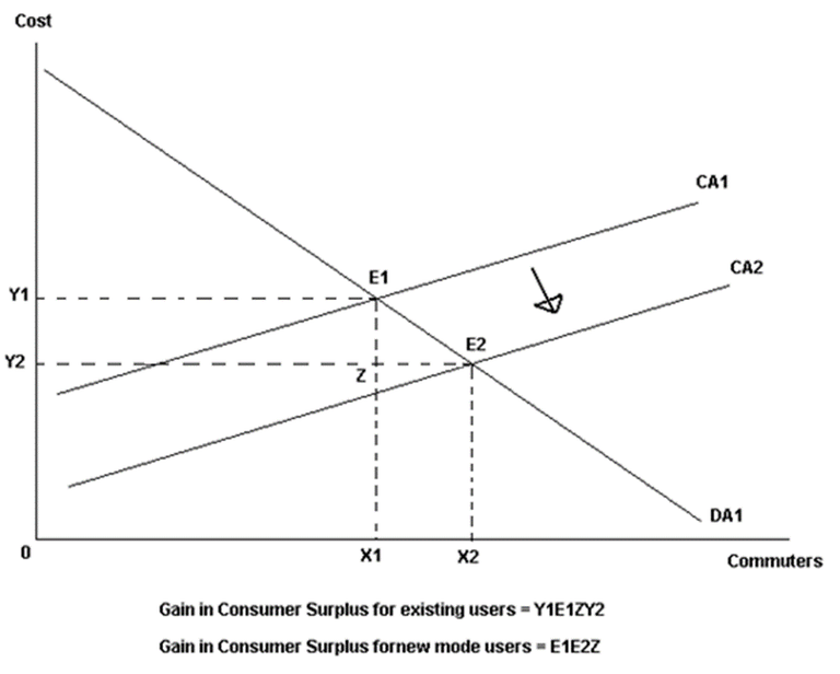
Figure 4: Cost Savings from Reduced Demand
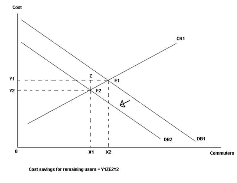
Where:
CA1 = perceived cost of Mode A before initiative
CA2 = perceived cost of Mode A after initiative
DA1 = demand for Mode A
CB1 = perceived cost of Mode B
DB1 = demand for Mode B before initiative
DB2 = demand for Mode B after initiative
The difference between X1 and X2 are the number of commuters switching between modes. The benefits calculated for commuters switching mode is dependent on the elasticity of demand for the mode commuters are switching to and the extent of the perceived cost savings.
The model demonstrated in Figures 3 and 4 is dependent upon linear demand functions for both modes of transport and a consistent perception of costs. The Tri Methodology assumes multiple perceived cost functions. Figure 5 provides a brief overview of the perceived costs of a group of commuters.
Figure 5: Cost Savings for Commuter Group X using the Tri Methodology
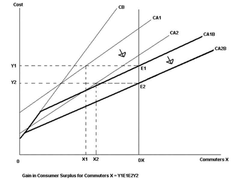
Where:
CA1B = combined perceived costs of two competing modes before initiative
CA2B = combined perceived costs of two competing modes after initiative
The demand function is perfectly inelastic based on the assumption that there is no generated or induced demand for commuter Group X. Consistent with the approach described in Figure 3, X2-X1 commuters have switched mode. The savings/benefits to each commuter in Group X is the same regardless of mode of transport used; this assumption has been made as commuters within this group are assumed to transfer to the mode with reduced perceived cost savings until commuters in Group X are indifferent between the two modes. This approach is then repeated for all commuter groups to derive total costs savings across all groups.
The model described in Figure 5 is subject to the assumption of perfect mobility between modes of transport. In reality, many commuters cannot easily switch between modes. This problem can be resolved by assuming a fixed percentage of commuters are committed to a particular mode of transport regardless of changes in perceived costs.
7. APPLICATIONS OF THE TRI METHODOLOGY
Queensland Transport and Main Road (TMR) have applied the Tri Methodology to determine the benefits of non-infrastructure initiatives in the absence of detailed modelling. The Triangle multi-modal (TRIMM) model was completed in 2013 to be used in-house by TMR (TMR 2013a). TRIMM is expected to primarily be used to evaluate the benefits of non-infrastructure alternatives to urban infrastructure projects. As the non-infrastructure option will be considered among many infrastructure solutions, sufficient time and resources will not be available for the dedicated modelling of the outcomes of the non-infrastructure option.
The TRIMM model was tested and compared with a spreadsheet using typical outputs from the Brisbane Strategic Transport Model (BSTM) (TMR 2013b) for a flexible working hours initiative for Brisbane. The benefits calculated using the TRIMM model were within 15% of those calculated using the spreadsheet and BSTM outputs. This test provided an indication that the model can produce reasonably reliable results. However, one test is not sufficient to declare the model a success. The model has also been peer reviewed by several experts that found it to be sound. The outputs produced from the model will continue to undergo scrutiny to check for errors. Figure 6 contains the input interface of TRIMM displaying an example of the impact of increased frequency of bus services.
Figure 6: Input Interface of TRIMM
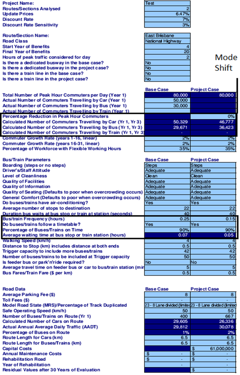
In this example, the frequency of bus services for a particular area has been proposed to improve from an average of every 15 minutes (0.25) to every 9 minutes (0.15) per bus per service. The increased number of buses will reduce time waiting at bus stops and reduce crowding on buses. The perceived costs for travelling by bus has been reduced, hence causing a mode shift from car to bus. In the example in Figure 6, the daily peak bus patronage has been calculated to increase from 29,671 in year 1 to 36,432 in year 3 while the number of commuters using cars has dropped from 50,329 in year 1 to 46,777 in year 3.
For the TRIMM model, mode shift is also influenced by changes in the other available inputs in the interface shown in Figure 6 but to varying extent. For example, cleaner buses will result in less of a mode shift than a 30% decrease in bus fares assuming existing buses have the capacity to cater for the mode shift. TRIMM also includes the option to include a fixed percentage of commuters who will not shift mode regardless of any initiative. Table 1, contains the summary of results produced by TRIMM for the example of increased bus service frequency.
Table 1: Results Produced by TRIMM for Example of Increased Bus Service Frequency.
Results 4% 7% 10%
Total Costs $ 26,347,122 $ 33,894,462 $ 39,531,592
Capital Costs $ 61,000,000 $ 61,000,000 $ 61,000,000
Maintenance/Rehabilitation $ - $ - $ -
Net Cost of New Buses and Trains -$ 34,652,878 -$ 27,105,538 -$ 21,468,408
Total Benefits $ 125,153,341 $ 85,442,489 $ 60,116,908
Travel Time Cost Savings $ 98,606,692 $ 65,870,130 $ 45,270,494
Vehicle Operating Cost Savings $ 21,952,154 $ 16,216,294 $ 12,324,974
Accident Cost Savings $ 1,421,612 $ 1,067,558 $ 822,786
Emission Cost Savings $ 1,833,745 $ 1,333,450 $ 999,283
Other Externality Cost Savings $ 1,339,138 $ 955,056 $ 699,371
Net Present Value (NPV) $ 98,806,219 $ 51,548,027 $ 20,585,316
Benefit Cost Ratio (BCR) 4.75 2.52 1.52
Net Benefit Investment Ratio (NBIR) 2.62 1.85 1.34
Additional Information Total TTC & VOC Savings $ 120,558,846 $ 82,086,424 $ 57,595,469
TTC & VOC Savings (Cars) $ 165,550,444 $ 119,899,794 $ 89,506,906
TTC & VOC Savings (Buses) -$ 44,991,598 -$ 37,813,370 -$ 31,911,437
TTC & VOC Savings (Trains) $ - $ - $ -
Discounted Revenue (Increase) -$ 22,467,099 -$ 29,458,805 -$ 41,152,118
Revenue from Bus Fares $ 50,153,828 $ 65,761,574 $ 91,864,829
Revenue from Tolls $ - $ - $ -
Revenue from Parking -$ 72,620,927 -$ 95,220,379 -$ 133,016,946
Revenue from Train Fares $ - $ - $ -
The results are presented using a typical TMR layout of three discount rates with benefits broken down into the four core benefit categories of travel time cost (TTC), vehicle operating cost (VOC), accident cost and emission cost savings (TMR 2011). The benefits for the four categories have been calculated using the Austroads (2005) algorithms. Typical economic indicators such as net present value (NPV) and benefit cost ratio (BCR) are also included. The results also include additional information such as cost savings and discounted changes in revenue for each mode of transport. Breaking cost savings down according to new and existing users for each mode is an expected inclusion for the next version of the model.
The differences in unperceived costs between modes of transport are the fundamental source of benefits for most of the non-infrastructure solutions evaluated using TRIMM. Many non-infrastructure solutions aim to influence perceived costs to compensate for some of the unperceived costs. TRIMM captures the changes in perceived costs and the corresponding effect on commuter behaviour, which ultimately affects commuter travel costs. Both perceived and unperceived costs are incorporated in the results presented in TRIMM, where possible, over-perceived costs are excluded from the results.
8. CONCLUSION
The methodology described in this paper to determine mode shift in the absence of detailed modelling, Tri Methodology, has been kept reasonably simple. The Tri Methodology can be incorporated into spreadsheets and models to evaluate the benefits of any initiatives that are expected to influence perceived costs and cause mode shifts. The ideal use of the Tri Methodology is at the early planning stages such as during the options analysis of proposed initiatives as a gauge of the likely benefits produced by options. Once options have been eliminated, detailed modelling should still be considered the most appropriate course of action if time and resources permit. The methodology is not intended to be a preferred substitute to detailed modelling but an alternative when such modelling is not available or feasible.
So far, the Tri Methodology has been applied to the triangle multi-modal (TRIMM) non-infrastructure model for internal use in TMR. The methodology suits the requirements of the model and has been used to produce projected streams of benefits for non-infrastructure initiatives expected to cause mode shifts. The application of the Tri Methodology need not be restricted to non-infrastructure models but can be applied to any model that evaluates initiatives that are likely to cause transport mode shifts.
END NOTES
- Rightward shift in cost curves or distributions indicates an increase in costs (Begg, Fischer and Dornbusch 2000).
- The Tri Methodology need not be confined to the perceived cost formulae provided by the ATC guidelines but to any formulae that provides sensitivities to various perceived cost components.
- The iterations represent the various possible combinations of distributions that have been combined to derive the most representative breakdown of current mode use using model parameters.
- For simplicity, concessions have been excluded.
- Parking fees can vary between car parks and season parking may not but be fully realised.
- The numerator of the equation is the calculation of the peak of the triangle using the area of the triangle, which is assumed equal to the total number of commuters.
- Formulae in Equations 7 to 10 can also be expressed be calculating the area of the triangles using ½ height × width. The calculus version was used in the paper so that the methodology can be applied to distributions other than the triangle distribution.
- Consumer surplus is the difference between the amount the consumer is willing to pay for a commodity and the amount that is actually paid (Maunder et al 1995).
- The values relate to the changes in costs for the mode and do not reflect cost savings to new or existing users for that particular mode. In hindsight, this inclusion could create confusion regarding the distribution of cost savings.
REFERENCES
Australian Transport Council (2006), National Guidelines for Transport Systems Management in Australia, 4 Urban Transport, Commonwealth of Australia, Canberra.
Austroads (2012), Guide to Project Evaluation – Part 4: Project Evaluation Data (Updated Road User Effects Unit Values), Austroads.
Austroads (2005), Economic Evaluation of Road Investment Proposals: Harmonisation of Non-urban Road User Cost Models, Austroads, AP-R264/05.
Begg, D., Fischer, S. and Dornbusch, R. (2000), Economics 6th Edition, McGraw Hill, London.
Damodaran, A. (2007), Statistical Distributions, Dama odaran Online,available at http://pages.stern.nyu.edu/~adamodar/New_Home_Page/StatFile, accessed 31/10/2013.
Department for Transport (2014a), TAG Unit M3.1: Highway Assignment Modelling, Transport Analysis Guidance, Department for Transport.
Department for Transport (2014b), TAG Unit M3.2: Public Transport Assignment Modelling, Transport Analysis Guidance, Department for Transport.
Hausman, J. A. and Wise, D. A., (1976), A Conditional Probit Model for Qualitative Choice: Discrete Decisions Recognizing Interdependence and Heterogenous Preferences, Massachusetts Institute of Technology, 173.
Maunder, P., Myers, D., Wall, N., and Miller, R. L., (1995), Economics Explained Third Edition, Collins Educational Publishers, London.
NZ Transport Agency (2010), Economic Evaluation Manual (Volume 2), NZ Transport Agency.
Transport and Main Roads (2013a), Triangular Multi-modal Model Methodology, Queensland Government (Unpublished).
Transport and Main Roads (2013b), Travel Demand Management (TDM) Flexible Working Hours – Rapid Cost Benefit Analysis, Queensland Government (Unpublished).
Transport and Main Roads (2011), Cost-benefit Analysis Manual: Road Projects, Queensland Government, Brisbane.
TRT Trasporti e Trerritorio SRL (2012), TRACECA Appraisal Manual Guidelines for Pre-Feasibility of Transport Projects with Exercises and Case Studies, Interoperability and Dialogue between Europe and Asia (IDEA).
Equation 9
RUBB>0 = MeanB∫MinB(α1P+β1PXP)dx + Min(MaxP, MaxB)∫MeanB(α2P+β2PXP)dx
Equation 107
RUP = RUPB=0 + (RUT – RUPB=0) × RUPB>0/(RUPB>0 + RUBB>0)
Where:
RUP = commuters travelling by private car
RUPB>0 = maximum number of commuters that could travel by private car when probability of travelling by bus is greater than zero
RUBB>0 = maximum number of commuters that could travel by bus when probability of travelling by bus is greater than zero and the probability of travelling by private car is less than one
RUPB=0 = commuters travelling by private car when probability of travelling by bus is zero
RUT = Total number of commuters
XP/B = perceived costs of using private cars or buses
MeanP = mean perceived costs of using private cars
MinP = minimum perceived costs of using private cars
MaxP = maximum perceived costs of using private cars
MeanB = mean perceived costs of using buses
MinB = minimum perceived costs of using buses
MaxB = maximum perceived costs of using buses
The commuters travelling by bus (RUB) can be calculated by subtracting commuters travelling by private car (RUP) from the total number of commuters (RUT). Equations 7 to 10 hold true if the minimum perceived cost for travelling by private car is less than the minimum perceived cost for travelling by bus. If the perceived cost for travelling by bus is less than that of travelling by private car, Equations 7 to 10 can be applied to calculate the number of commuters expected to travel by bus by substituting the parameters for private cars with those for buses. RUP can be calculated by subtracting RUB from RUT.
The number of cars expected on the road can easily be calculated by dividing RUP by the average occupancy of private cars. The number of buses on the route can be considered predetermined but dividing RUB by the number of buses will provide an estimate of the average occupancy of buses.
If the results from the model are not consistent with actual data, the minimum, maximum and mean perceived costs can be adjusted to determine a range of feasible minimum, maximum and mean perceived costs that produce results close to that of the actual data. Once the traffic volumes are consistent, the model can be used to predict changes in commuter behaviour from infrastructure upgrades resulting in improved reliability or reduced road congestion or policy changes such as changes in tolls, average parking fees, bus fares, or increased frequency of buses.
The application of the triangle distribution of perceived costs has been discussed in the context of buses and private cars, the rail component is a less detailed extension of the theory. To incorporate rail, three comparisons are made using the triangle distributions, they are buses with cars, buses with trains, and trains with cars. A weighted average of the outputs produced through the comparisons of the distributions is used as an approximation of mode choice. The alternative of directly adding a third triangle to the distributions would require a more complicated extension to the model.
5. TREATMENT OF UNPERCEIVED COSTS
Perceived costs have been used to determine the behaviour and choice of mode of transport for commuters. Unperceived costs are costs that do not influence the commuters’ choice of mode as they are not recognised by the commuter (Department for Transport 2014b) but should still be considered in an analysis. The unperceived costs for commuting with private cars tend to be quite high in comparison to the unperceived costs of using public transport (NZ Transport Agency 2010). The unperceived costs included in the methodology for private cars are oil, vehicle depreciation, large portion of tyre wear costs, repair and maintenance of vehicle, accident costs, and emissions and other vehicle produced externalities. Some costs for some commuters may even be over-perceived such as fuel costs, which includes fuel tax. The unperceived costs of using public transport has been restricted to just inflexible or unreliable bus and train arrivals and emission and externalities produced by public transport. Commuters are also more susceptible to over-perceive the costs of using public transport. Such over-perceived costs include comfort and convenience, waiting at bus stops or train stations, facilities at train stations, and bus and train fares.
6. APPROACHES TO CHANGES IN CONSUMER SURPLUS8
Gains in consumer surplus from additional commuters using a mode have not been considered in the Tri Methodology. There are two reasons why the gains in consumer surplus of additional commuters to a mode were not considered. Generated or induced demand has not been considered in the model, the inclusion was deemed beyond the scope of what the methodology was trying to achieve. Benefits for all commuters are calculated directly as cost savings rather than gains in consumer surplus from mode shifts. The application of consumer surplus would normally involve perceived commuter cost savings for a particular mode of transport. These cost savings would induce commuters from another mode of transport (Mode B) to switch to the mode of transport with the perceived cost savings (Mode A). The benefits to commuters switching mode of transport is calculated as the gain in consumer surplus. Commuters not switching to Mode A still benefit from reduced costs from additional capacity on Mode B created by the commuters that switched. Gains in consumer surplus for those using Mode A are demonstrated in Figure 3 and savings to those remaining with Mode B is shown Figure 4.
Figure 3: Changes in Consumer Surplus

Figure 4: Cost Savings from Reduced Demand

Where:
CA1 = perceived cost of Mode A before initiative
CA2 = perceived cost of Mode A after initiative
DA1 = demand for Mode A
CB1 = perceived cost of Mode B
DB1 = demand for Mode B before initiative
DB2 = demand for Mode B after initiative
The difference between X1 and X2 are the number of commuters switching between modes. The benefits calculated for commuters switching mode is dependent on the elasticity of demand for the mode commuters are switching to and the extent of the perceived cost savings.
The model demonstrated in Figures 3 and 4 is dependent upon linear demand functions for both modes of transport and a consistent perception of costs. The Tri Methodology assumes multiple perceived cost functions. Figure 5 provides a brief overview of the perceived costs of a group of commuters.
Figure 5: Cost Savings for Commuter Group X using the Tri Methodology

Where:
CA1B = combined perceived costs of two competing modes before initiative
CA2B = combined perceived costs of two competing modes after initiative
The demand function is perfectly inelastic based on the assumption that there is no generated or induced demand for commuter Group X. Consistent with the approach described in Figure 3, X2-X1 commuters have switched mode. The savings/benefits to each commuter in Group X is the same regardless of mode of transport used; this assumption has been made as commuters within this group are assumed to transfer to the mode with reduced perceived cost savings until commuters in Group X are indifferent between the two modes. This approach is then repeated for all commuter groups to derive total costs savings across all groups.
The model described in Figure 5 is subject to the assumption of perfect mobility between modes of transport. In reality, many commuters cannot easily switch between modes. This problem can be resolved by assuming a fixed percentage of commuters are committed to a particular mode of transport regardless of changes in perceived costs.
7. APPLICATIONS OF THE TRI METHODOLOGY
Queensland Transport and Main Road (TMR) have applied the Tri Methodology to determine the benefits of non-infrastructure initiatives in the absence of detailed modelling. The Triangle multi-modal (TRIMM) model was completed in 2013 to be used in-house by TMR (TMR 2013a). TRIMM is expected to primarily be used to evaluate the benefits of non-infrastructure alternatives to urban infrastructure projects. As the non-infrastructure option will be considered among many infrastructure solutions, sufficient time and resources will not be available for the dedicated modelling of the outcomes of the non-infrastructure option.
The TRIMM model was tested and compared with a spreadsheet using typical outputs from the Brisbane Strategic Transport Model (BSTM) (TMR 2013b) for a flexible working hours initiative for Brisbane. The benefits calculated using the TRIMM model were within 15% of those calculated using the spreadsheet and BSTM outputs. This test provided an indication that the model can produce reasonably reliable results. However, one test is not sufficient to declare the model a success. The model has also been peer reviewed by several experts that found it to be sound. The outputs produced from the model will continue to undergo scrutiny to check for errors. Figure 6 contains the input interface of TRIMM displaying an example of the impact of increased frequency of bus services.
Figure 6: Input Interface of TRIMM

In this example, the frequency of bus services for a particular area has been proposed to improve from an average of every 15 minutes (0.25) to every 9 minutes (0.15) per bus per service. The increased number of buses will reduce time waiting at bus stops and reduce crowding on buses. The perceived costs for travelling by bus has been reduced, hence causing a mode shift from car to bus. In the example in Figure 6, the daily peak bus patronage has been calculated to increase from 29,671 in year 1 to 36,432 in year 3 while the number of commuters using cars has dropped from 50,329 in year 1 to 46,777 in year 3.
For the TRIMM model, mode shift is also influenced by changes in the other available inputs in the interface shown in Figure 6 but to varying extent. For example, cleaner buses will result in less of a mode shift than a 30% decrease in bus fares assuming existing buses have the capacity to cater for the mode shift. TRIMM also includes the option to include a fixed percentage of commuters who will not shift mode regardless of any initiative. Table 1, contains the summary of results produced by TRIMM for the example of increased bus service frequency.
Table 1: Results Produced by TRIMM for Example of Increased Bus Service Frequency.
Results 4% 7% 10%
Total Costs $ 26,347,122 $ 33,894,462 $ 39,531,592
Capital Costs $ 61,000,000 $ 61,000,000 $ 61,000,000
Maintenance/Rehabilitation $ - $ - $ -
Net Cost of New Buses and Trains -$ 34,652,878 -$ 27,105,538 -$ 21,468,408
Total Benefits $ 125,153,341 $ 85,442,489 $ 60,116,908
Travel Time Cost Savings $ 98,606,692 $ 65,870,130 $ 45,270,494
Vehicle Operating Cost Savings $ 21,952,154 $ 16,216,294 $ 12,324,974
Accident Cost Savings $ 1,421,612 $ 1,067,558 $ 822,786
Emission Cost Savings $ 1,833,745 $ 1,333,450 $ 999,283
Other Externality Cost Savings $ 1,339,138 $ 955,056 $ 699,371
Net Present Value (NPV) $ 98,806,219 $ 51,548,027 $ 20,585,316
Benefit Cost Ratio (BCR) 4.75 2.52 1.52
Net Benefit Investment Ratio (NBIR) 2.62 1.85 1.34
Additional Information Total TTC & VOC Savings $ 120,558,846 $ 82,086,424 $ 57,595,469
TTC & VOC Savings (Cars) $ 165,550,444 $ 119,899,794 $ 89,506,906
TTC & VOC Savings (Buses) -$ 44,991,598 -$ 37,813,370 -$ 31,911,437
TTC & VOC Savings (Trains) $ - $ - $ -
Discounted Revenue (Increase) -$ 22,467,099 -$ 29,458,805 -$ 41,152,118
Revenue from Bus Fares $ 50,153,828 $ 65,761,574 $ 91,864,829
Revenue from Tolls $ - $ - $ -
Revenue from Parking -$ 72,620,927 -$ 95,220,379 -$ 133,016,946
Revenue from Train Fares $ - $ - $ -
The results are presented using a typical TMR layout of three discount rates with benefits broken down into the four core benefit categories of travel time cost (TTC), vehicle operating cost (VOC), accident cost and emission cost savings (TMR 2011). The benefits for the four categories have been calculated using the Austroads (2005) algorithms. Typical economic indicators such as net present value (NPV) and benefit cost ratio (BCR) are also included. The results also include additional information such as cost savings and discounted changes in revenue for each mode of transport. Breaking cost savings down according to new and existing users for each mode is an expected inclusion for the next version of the model.
The differences in unperceived costs between modes of transport are the fundamental source of benefits for most of the non-infrastructure solutions evaluated using TRIMM. Many non-infrastructure solutions aim to influence perceived costs to compensate for some of the unperceived costs. TRIMM captures the changes in perceived costs and the corresponding effect on commuter behaviour, which ultimately affects commuter travel costs. Both perceived and unperceived costs are incorporated in the results presented in TRIMM, where possible, over-perceived costs are excluded from the results.
8. CONCLUSION
The methodology described in this paper to determine mode shift in the absence of detailed modelling, Tri Methodology, has been kept reasonably simple. The Tri Methodology can be incorporated into spreadsheets and models to evaluate the benefits of any initiatives that are expected to influence perceived costs and cause mode shifts. The ideal use of the Tri Methodology is at the early planning stages such as during the options analysis of proposed initiatives as a gauge of the likely benefits produced by options. Once options have been eliminated, detailed modelling should still be considered the most appropriate course of action if time and resources permit. The methodology is not intended to be a preferred substitute to detailed modelling but an alternative when such modelling is not available or feasible.
So far, the Tri Methodology has been applied to the triangle multi-modal (TRIMM) non-infrastructure model for internal use in TMR. The methodology suits the requirements of the model and has been used to produce projected streams of benefits for non-infrastructure initiatives expected to cause mode shifts. The application of the Tri Methodology need not be restricted to non-infrastructure models but can be applied to any model that evaluates initiatives that are likely to cause transport mode shifts.
END NOTES
- Rightward shift in cost curves or distributions indicates an increase in costs (Begg, Fischer and Dornbusch 2000).
- The Tri Methodology need not be confined to the perceived cost formulae provided by the ATC guidelines but to any formulae that provides sensitivities to various perceived cost components.
- The iterations represent the various possible combinations of distributions that have been combined to derive the most representative breakdown of current mode use using model parameters.
- For simplicity, concessions have been excluded.
- Parking fees can vary between car parks and season parking may not but be fully realised.
- The numerator of the equation is the calculation of the peak of the triangle using the area of the triangle, which is assumed equal to the total number of commuters.
- Formulae in Equations 7 to 10 can also be expressed be calculating the area of the triangles using ½ height × width. The calculus version was used in the paper so that the methodology can be applied to distributions other than the triangle distribution.
- Consumer surplus is the difference between the amount the consumer is willing to pay for a commodity and the amount that is actually paid (Maunder et al 1995).
- The values relate to the changes in costs for the mode and do not reflect cost savings to new or existing users for that particular mode. In hindsight, this inclusion could create confusion regarding the distribution of cost savings.
REFERENCES
Australian Transport Council (2006), National Guidelines for Transport Systems Management in Australia, 4 Urban Transport, Commonwealth of Australia, Canberra.
Austroads (2012), Guide to Project Evaluation – Part 4: Project Evaluation Data (Updated Road User Effects Unit Values), Austroads.
Austroads (2005), Economic Evaluation of Road Investment Proposals: Harmonisation of Non-urban Road User Cost Models, Austroads, AP-R264/05.
Begg, D., Fischer, S. and Dornbusch, R. (2000), Economics 6th Edition, McGraw Hill, London.
Damodaran, A. (2007), Statistical Distributions, Dama odaran Online,available at http://pages.stern.nyu.edu/~adamodar/New_Home_Page/StatFile, accessed 31/10/2013.
Department for Transport (2014a), TAG Unit M3.1: Highway Assignment Modelling, Transport Analysis Guidance, Department for Transport.
Department for Transport (2014b), TAG Unit M3.2: Public Transport Assignment Modelling, Transport Analysis Guidance, Department for Transport.
Hausman, J. A. and Wise, D. A., (1976), A Conditional Probit Model for Qualitative Choice: Discrete Decisions Recognizing Interdependence and Heterogenous Preferences, Massachusetts Institute of Technology, 173.
Maunder, P., Myers, D., Wall, N., and Miller, R. L., (1995), Economics Explained Third Edition, Collins Educational Publishers, London.
NZ Transport Agency (2010), Economic Evaluation Manual (Volume 2), NZ Transport Agency.
Transport and Main Roads (2013a), Triangular Multi-modal Model Methodology, Queensland Government (Unpublished).
Transport and Main Roads (2013b), Travel Demand Management (TDM) Flexible Working Hours – Rapid Cost Benefit Analysis, Queensland Government (Unpublished).
Transport and Main Roads (2011), Cost-benefit Analysis Manual: Road Projects, Queensland Government, Brisbane.
TRT Trasporti e Trerritorio SRL (2012), TRACECA Appraisal Manual Guidelines for Pre-Feasibility of Transport Projects with Exercises and Case Studies, Interoperability and Dialogue between Europe and Asia (IDEA).
RUP = RUPB=0 + (RUT – RUPB=0) × RUPB>0/(RUPB>0 + RUBB>0)
RUP = commuters travelling by private car
RUPB>0 = maximum number of commuters that could travel by private car when probability of travelling by bus is greater than zero
RUBB>0 = maximum number of commuters that could travel by bus when probability of travelling by bus is greater than zero and the probability of travelling by private car is less than one
RUPB=0 = commuters travelling by private car when probability of travelling by bus is zero
RUT = Total number of commuters
XP/B = perceived costs of using private cars or buses
MeanP = mean perceived costs of using private cars
MinP = minimum perceived costs of using private cars
MaxP = maximum perceived costs of using private cars
MeanB = mean perceived costs of using buses
MinB = minimum perceived costs of using buses
MaxB = maximum perceived costs of using buses


CA1 = perceived cost of Mode A before initiative
CA2 = perceived cost of Mode A after initiative
DA1 = demand for Mode A
CB1 = perceived cost of Mode B
DB1 = demand for Mode B before initiative
DB2 = demand for Mode B after initiative

CA1B = combined perceived costs of two competing modes before initiative
CA2B = combined perceived costs of two competing modes after initiative

Results| 4% | 7% | 10%
| Total Costs | $ 26,347,122 | $ 33,894,462 | $ 39,531,592
| Capital Costs | $ 61,000,000 | $ 61,000,000 | $ 61,000,000
| Maintenance/Rehabilitation | $ - | $ - | $ -
| Net Cost of New Buses and Trains | -$ 34,652,878 | -$ 27,105,538 | -$ 21,468,408
|
| Total Benefits | $ 125,153,341 | $ 85,442,489 | $ 60,116,908
| Travel Time Cost Savings | $ 98,606,692 | $ 65,870,130 | $ 45,270,494
| Vehicle Operating Cost Savings | $ 21,952,154 | $ 16,216,294 | $ 12,324,974
| Accident Cost Savings | $ 1,421,612 | $ 1,067,558 | $ 822,786
| Emission Cost Savings | $ 1,833,745 | $ 1,333,450 | $ 999,283
| Other Externality Cost Savings | $ 1,339,138 | $ 955,056 | $ 699,371
|
| Net Present Value (NPV) | $ 98,806,219 | $ 51,548,027 | $ 20,585,316
| Benefit Cost Ratio (BCR) | 4.75 | 2.52 | 1.52
| Net Benefit Investment Ratio (NBIR) | 2.62 | 1.85 | 1.34
|
| Additional Information |
| Total TTC & VOC Savings | $ 120,558,846 | $ 82,086,424 | $ 57,595,469
| TTC & VOC Savings (Cars) | $ 165,550,444 | $ 119,899,794 | $ 89,506,906
| TTC & VOC Savings (Buses) | -$ 44,991,598 | -$ 37,813,370 | -$ 31,911,437
| TTC & VOC Savings (Trains) | $ - | $ - | $ -
|
| Discounted Revenue (Increase) | -$ 22,467,099 | -$ 29,458,805 | -$ 41,152,118
| Revenue from Bus Fares | $ 50,153,828 | $ 65,761,574 | $ 91,864,829
| Revenue from Tolls | $ - | $ - | $ -
| Revenue from Parking | -$ 72,620,927 | -$ 95,220,379 | -$ 133,016,946
| Revenue from Train Fares | $ - | $ - | $ - |
The results are presented using a typical TMR layout of three discount rates with benefits broken down into the four core benefit categories of travel time cost (TTC), vehicle operating cost (VOC), accident cost and emission cost savings (TMR 2011). The benefits for the four categories have been calculated using the Austroads (2005) algorithms. Typical economic indicators such as net present value (NPV) and benefit cost ratio (BCR) are also included. The results also include additional information such as cost savings and discounted changes in revenue for each mode of transport. Breaking cost savings down according to new and existing users for each mode is an expected inclusion for the next version of the model. The differences in unperceived costs between modes of transport are the fundamental source of benefits for most of the non-infrastructure solutions evaluated using TRIMM. Many non-infrastructure solutions aim to influence perceived costs to compensate for some of the unperceived costs. TRIMM captures the changes in perceived costs and the corresponding effect on commuter behaviour, which ultimately affects commuter travel costs. Both perceived and unperceived costs are incorporated in the results presented in TRIMM, where possible, over-perceived costs are excluded from the results. 8. CONCLUSIONThe methodology described in this paper to determine mode shift in the absence of detailed modelling, Tri Methodology, has been kept reasonably simple. The Tri Methodology can be incorporated into spreadsheets and models to evaluate the benefits of any initiatives that are expected to influence perceived costs and cause mode shifts. The ideal use of the Tri Methodology is at the early planning stages such as during the options analysis of proposed initiatives as a gauge of the likely benefits produced by options. Once options have been eliminated, detailed modelling should still be considered the most appropriate course of action if time and resources permit. The methodology is not intended to be a preferred substitute to detailed modelling but an alternative when such modelling is not available or feasible. So far, the Tri Methodology has been applied to the triangle multi-modal (TRIMM) non-infrastructure model for internal use in TMR. The methodology suits the requirements of the model and has been used to produce projected streams of benefits for non-infrastructure initiatives expected to cause mode shifts. The application of the Tri Methodology need not be restricted to non-infrastructure models but can be applied to any model that evaluates initiatives that are likely to cause transport mode shifts. END NOTES
REFERENCESAustralian Transport Council (2006), National Guidelines for Transport Systems Management in Australia, 4 Urban Transport, Commonwealth of Australia, Canberra. Austroads (2012), Guide to Project Evaluation – Part 4: Project Evaluation Data (Updated Road User Effects Unit Values), Austroads. Austroads (2005), Economic Evaluation of Road Investment Proposals: Harmonisation of Non-urban Road User Cost Models, Austroads, AP-R264/05. Begg, D., Fischer, S. and Dornbusch, R. (2000), Economics 6th Edition, McGraw Hill, London. Damodaran, A. (2007), Statistical Distributions, Dama odaran Online,available at http://pages.stern.nyu.edu/~adamodar/New_Home_Page/StatFile, accessed 31/10/2013. Department for Transport (2014a), TAG Unit M3.1: Highway Assignment Modelling, Transport Analysis Guidance, Department for Transport. Department for Transport (2014b), TAG Unit M3.2: Public Transport Assignment Modelling, Transport Analysis Guidance, Department for Transport. Hausman, J. A. and Wise, D. A., (1976), A Conditional Probit Model for Qualitative Choice: Discrete Decisions Recognizing Interdependence and Heterogenous Preferences, Massachusetts Institute of Technology, 173. Maunder, P., Myers, D., Wall, N., and Miller, R. L., (1995), Economics Explained Third Edition, Collins Educational Publishers, London. NZ Transport Agency (2010), Economic Evaluation Manual (Volume 2), NZ Transport Agency. Transport and Main Roads (2013a), Triangular Multi-modal Model Methodology, Queensland Government (Unpublished). Transport and Main Roads (2013b), Travel Demand Management (TDM) Flexible Working Hours – Rapid Cost Benefit Analysis, Queensland Government (Unpublished). Transport and Main Roads (2011), Cost-benefit Analysis Manual: Road Projects, Queensland Government, Brisbane. TRT Trasporti e Trerritorio SRL (2012), TRACECA Appraisal Manual Guidelines for Pre-Feasibility of Transport Projects with Exercises and Case Studies, Interoperability and Dialogue between Europe and Asia (IDEA). |
|---|
Congratulations @spectrumecons! You have completed the following achievement on the Hive blockchain And have been rewarded with New badge(s)
Your next payout target is 100000 HP.
The unit is Hive Power equivalent because post and comment rewards can be split into HP and HBD
You can view your badges on your board and compare yourself to others in the Ranking
If you no longer want to receive notifications, reply to this comment with the word
STOP