If you are familiar with the MATCH function in Excel then you are going to love XMATCH. Just like the MATCH function XMATCH returns a relative position in a list. Now you are familiar XLOOKUP, which replaces the old VLOOKUP function, you know XLOOKUP comes with additional power. This come in the form of new conditions in the formula syntax such as search mode and match types. Well, XMATCH also as this extra power over its predecessor MATCH.
XMATCH is available in Excel/Office 365
The syntax for XMATCH is
XMATCH(Lookup Value, Lookup Array, [Match Mode],[Search Mode])
Where:
Lookup Value is the value you are looking to find the relative position
Lookup Array is the row or column that contains the Lookup Value
Match mode is optional. Unlike the old MATCH function, the default is an exact match. You can also select between
- Exact match or next smallest
- Exact match or next largest
- Wildcard match
XMATCH – The Basics
We have a list of runners sorted by fastest to slowest. We wish to find the position of the selected runner.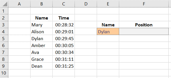
For this we can use the formula
=XMATCH(E4,B3:B9)
Where E4 contains the lookup value and the lookup array is B3:B9
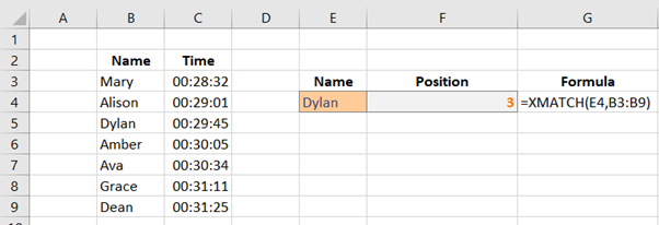
From this we can see that Dylan is the 3rd fastest.
We can also use the Match mode to search for Approximate matches. XMATCH allows us select between the next smallest or the next largest.
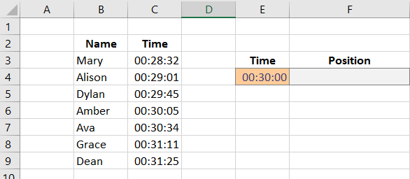
Given a time of 00:30:00 to search for the next smallest we will add -1 as the Match Mode.
=XMATCH(E4,C3:C9,-1)
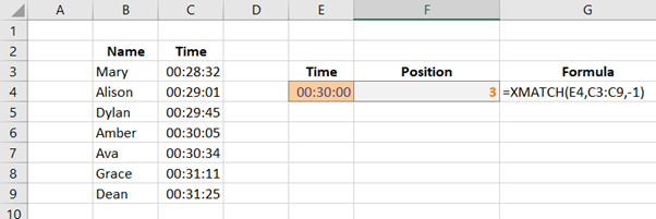
Given a time of 00:30:00 to search for the next largest we will add -1 as the Match Mode.
=XMATCH(E4,C3:C9,1)

The Match mode will also allow you to carry out a wildcard search. To do this, you must set the Match Mode to 2.
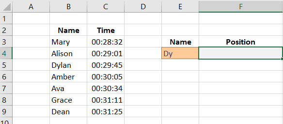
Assuming you only have the first two letters of a Name and we want to find the relative position.
We would use the formula
=XMATCH(E4&"*",B3:B9,2)
We must join the text from cell E4 with . To do this we use &””
And we select 2 for the Match mode.

INDEX and MATCH or INDEX and XMATCH
The MATCH function is often used with the INDEX function to create a lookup. XMATCH can be used in the same way. Let’s refresh quickly how INDEX and MATCH work together
INDEX returns an intercepting point. Its syntax is
INDEX(Array, row number, [column number])
When using INDEX and MATCH together, MATCH is used to generate the row and column numbers
For example, we want to look up the sales for Lisa in Apr using the INDEX and MATCH functions
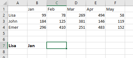
To do this we would use the following function
=INDEX(A1:F4,MATCH(A7,A1:A4,0),MATCH(B7,A1:F1,0))
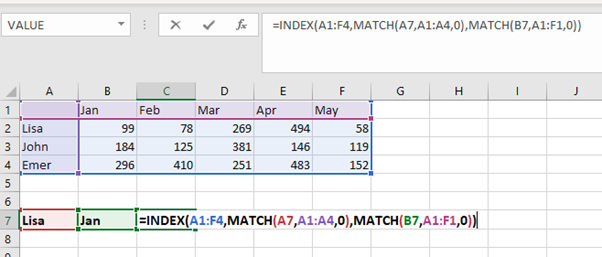
Using XMATCH we can carry out the same exercise. This time the formula would look as follows
=INDEX(A1:F4,XMATCH(A7,A1:A4),XMATCH(B7,A1:F1))

As you can see from the XMATCH, as the default is to search first to last, we do not need to add this to the formula, unlike when we were using MATCH.
Now it’s your turn – XMATCH in Excel
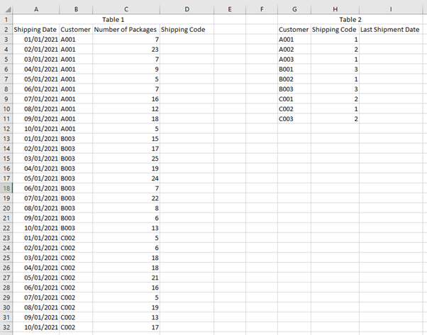
Your knowledge of INDEX and MATCH and XLOOKUP can be applied to XMATCH. Can you create a formula using XMATCH to return the following? You can download the data here
In table 1, column D, pull in the Shipping code from Table 2
In table 2, column I, pull in the last shipment date for each customer.
Share the formula you used for both in the comments below before you watch the video.
SIGN UP
Cross posted from my blog with SteemPress : https://theexcelclub.com/how-to-use-xmatch-in-excel/